Abstract
The Pilot Approximation Trajectory (PAT) contour algorithm can find the contour of a function accurately when it is not practical to evaluate the function on a grid dense enough to use a standard contour algorithm, for instance, when evaluating the function involves conducting a physical experiment or a computationally intensive simulation. PAT relies on an inexpensive pilot approximation to the function, such as interpolating from a sparse grid of inexact values, or solving a partial differential equation (PDE) numerically using a coarse discretization. For each level of interest, the location and 'trajectory' of an approximate contour of this pilot function are used to decide where to evaluate the original function to find points on its contour. Those points are joined by line segments to form the PAT approximation of the contour of the original function.
Approximating a contour numerically amounts to estimating a lower level set of the function, the set of points on which the function does not exceed the contour level. The area of the symmetric difference between the true lower level set and the estimated lower level set measures the accuracy of the contour. PAT measures its own accuracy by finding an upper confidence bound for this area.
In examples, PAT can estimate a contour more accurately than standard algorithms, using far fewer function evaluations than standard algorithms require. We illustrate PAT by constructing a confidence set for viscosity and thermal conductivity of a flowing gas from simulated noisy temperature measurements, a problem in which each evaluation of the function to be contoured requires solving a different set of coupled nonlinear PDEs.
1. Introduction
A contour, level curve, or isoline of a real-valued function of two variables is the set of points in the domain Δ of the function on which g takes one particular 'level' τ:


Contours are useful in many contexts, including visualizing geographical and meteorological data.
Typical contouring algorithms start with the values of g on a dense, regular grid. They approximate values of g between grid points by interpolation, usually linear interpolation (Cottafava and Moli 1969, McLain 1974, Aramini 1980). Work on efficiency in contouring algorithms primarily addresses large datasets; see, for example, Agarwal et al (2008) or van Kreveld et al (1997). For algorithms to construct contours in higher dimensions (iso-surfaces), see for example ( Bhaniramka et al 2004, Schreiner et al 2006). Contouring algorithms are closely related to algorithms for constructing level sets {x∈Δ:g(x) ⩾ τ}. Sethian (1999), Willett and Nowak (2005) and Scott and Davenport (2007) discuss efficient algorithms for approximating level sets.
We address a different bottleneck: finding approximate contours when it is very expensive to evaluate g. If g is expensive to evaluate and varies nonlinearly—for example, if each evaluation of g requires performing a physical experiment, running a computationally intensive simulation (as in climate modeling), or solving coupled nonlinear partial differential equations (PDEs) numerically—it can be impractical to evaluate g on a grid dense enough to approximate contours accurately using standard methods. To reiterate: we are not addressing contouring the solution to a single coupled nonlinear PDE problem on a two-dimensional domain. Rather, we are addressing the contouring of a function of two variables that for each value of a two-dimensional argument could require solving a different set of coupled nonlinear PDEs, or some other expensive calculation. The computational domain for the PDEs (typically a spatio-temporal domain) has no connection to the contour grid (a grid of parameter values).
Bryan et al (2006) and Bryan and Schneider (2008) describe an active learning algorithm for identifying contours of a function. Their algorithm uses statistical criteria to decide where to evaluate the function. In this paper, we describe a different approach: we use an approximation of the function as a starting point for an iterative search to locate the contour to any desired accuracy. We check the accuracy of the approximate contour by random sampling. The check does not require any assumptions about the function or the accuracy of the initial approximation (e.g., it does not require any regularity conditions on g).
In applications, particular contours such as the zero contour can be especially interesting. Examples are given below. In some such cases, an accurate approximate contour can be found using relatively few function evaluations by starting with an 'educated guess' about where the contour is—a pilot approximation—and then refining that approximation adaptively.
We present an algorithm that exploits this tactic, Pilot Approximation Trajectory (PAT). PAT contours at one level at a time. It takes advantage of the fact that g can be evaluated anywhere in Δ—albeit at a cost. By judiciously selecting where to evaluate g and avoiding evaluating g far from the level of interest, PAT requires fewer evaluations of g than standard contouring methods to attain the same accuracy—or better.
PAT starts by building a cheap pilot approximation of g. The pilot approximation might be constructed by interpolating values of g on sparse grid, for instance using splines. If evaluating g at a point requires solving a PDE numerically, might be the numerical solution based on a coarser discretization. In the latter case, note that the PDE discretization is in a different space from the contour grid: we are addressing problems where each evaluation of g requires solving a different PDE. The approximation involves solving each of those PDEs less accurately, not evaluating the solution to a single PDE at fewer points x. The pilot approximation is used to predict the location and trajectory (local orientation) of the contour, which are then refined by evaluating g at additional points. PAT treats g as a 'black box,' so it can estimate contours of complicated functions, including nondifferentiable functions involving real or simulated experiments.


To compare the performance of PAT to standard contouring algorithms requires quantifying the error of approximate contours. A contour divides the domain Δ into a set where g has values above the level τ and a set where the value of g is less than or equal to τ. The latter is called the lower level set of g (at level τ):

One can quantify accuracy of approximate contours based on how well they perform that classification—on how much the actual and estimated lower level sets differ, i.e., how well the approximate contour classifies points in Δ.
An approximate contour can make two kinds of classification errors: it can include values of g that are above the level, and it can fail to include values of g that are at or below the level. Let be the estimated lower level set of g at level τ according to the approximate contour. The first kind of error occurs on the set and the second kind of error occurs on the set . The union of these two sets, the points in the domain Δ that the approximate contour misclassifies, is the symmetric difference between and Λτ:


The area of this symmetric difference quantifies the error of the approximate contour. We compare PAT and standard contouring on the basis of their computational burden and on this measure of their accuracy in tests where the true contour is known. In practice, the true contour generally is not known. But PAT can use random sampling to find an upper confidence bound on the area of , assessing its own accuracy through additional evaluations of g.

The symmetric difference is not the only reasonable definition of the error of an approximate contour, even among measures based on the lower level set. For instance, if misclassifying some points in the domain has more serious consequences than misclassifying others, the fraction of the area of the domain on which the approximate contour errs might not be the most relevant measure of accuracy. One could use weighted areas to account for differing importance, for instance, integrals with respect to a measure other than the Lebesgue measure.
Measuring accuracy by the area of the symmetric difference between the true and approximate lower level sets is meaningful in applications. For instance, in one approach to uncertainty quantification, the ensemble of models method, Higdon (2010) rely on dividing the set of possible parameter values (models) into those that agree 'adequately' with the data and those that do not. Agreement is measured using a misfit function. The set of models that agree adequately with the data is a lower level set of the misfit function. In some problems, a lower level set of the misfit is a confidence set for the model that generated the data. Our motivating application is to find such a confidence set for a two-dimensional parameter from indirect, noisy measurements—an inverse problem. This is related to the example that motivates the work of Bryan et al (2006).
The paper is organized as follows. In the next subsection we give an example of a simple problem that motivates this work. Section 2 presents a basic version of PAT and a refinement to treat delicate cases, such as saddle points. It also discusses constructing confidence bounds on the fraction of the domain that the PAT contour correctly classifies as above or below the contour level. Section 3 applies PAT to two examples: contouring a function with a saddle point and finding a confidence set for viscosity and thermal conductivity from simulated data in an airflow inverse problem. Section 4 summarizes our findings.
1.1. A model problem: the heat equation
We consider a simple problem in which PAT is helpful: estimating the coefficients of a constant-coefficient steady state heat equation. The governing equation is

where a and b are the coefficients and h is a source term. This problem is two-dimensional in that the PDE depends on two coefficients; the domain of the PDE is three-dimensional. For example, the coefficients a and b might be parameters related to heat conductivity and perfusion; see Pennes (1948). We seek a 95% simultaneous confidence set for the unknown coefficients a and b based on observations y = (y1,...,yn)T from u,

where  is a n-vector representing observational noise and G = (G1,...,Gn)T represents the relationship between the observations and the underlying PDE. For example, G can be a linear interpolation operator which samples u of (4) in given measurement locations or it can be the negative temperature coefficient (NTC) resistor model. We assume that the components of are independent, identically distributed (iid) Gaussian variables with mean 0 and variance 1.
We will be contouring a function of , the vector of unknown parameters. Each value of x is a possible value for the coefficients in the heat equation, not a spatial location within the domain of the equation. Equation (5) has unique solution u for all positive x = (a,b) > 0. The solution can be approximated numerically, for example, using a finite-element method. Define the function f such that f(x) = G(u). That is, f maps a coefficient vector x = (a,b) into the n noise-free measurements according to the finite-element solution of (4) for coefficients x = (a,b). To evaluate f at a single point x = (a,b) requires finding the finite-element solution to equation (4) for the coefficients x = (a,b) and then applying the measurement model G to that finite-element solution.
The forward problem that maps a parameter vector to the observations thus can be written

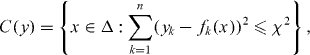
We want to find a confidence set for x with confidence level 95%. This is a set C(y) for which
whatever the true value x = (a,b) happens to be. An example of a 95% confidence set is
where the constant χ is chosen such that
The appendix gives more explanation.
The boundary of the confidence set C(y) is the level-χ contour of the function g(x) = . Evaluating g for a given parameter pair x = (a,b) can be expensive, especially if the problem is modeled in three spatial dimensions and the computational mesh contains large number of nodes. Regular contouring approaches might require evaluating g on a grid of 128 × 128 different parameter values, for instance. That would mean running the finite-element solver 1282 times, once for each of the 1282 parameter values. Clearly, it would be useful to be able to find the boundary of the confidence set with fewer evaluations of g; that is, the problem PAT addresses.
There are at least two ways to construct a pilot approximation for PAT:

- (i)Linear interpolation of g on a sparse grid. Evaluate g on a small grid of points (say 10 × 10 grid) in Δ. Divide each grid element into two triangles, forming a triangular tessellation of Δ. Set the pilot approximation to be the piecewise linear function equal to g at the nodes, linear within each triangle. (Instead of linear interpolation, one might use MARS (Friedman 1991) or a Gaussian process model (O'Hagan and Kingman 1978, Sacks et al 1989, Kennedy and O'Hagan 2001)).
- (ii)Solve the PDE at a low level of approximation for a dense grid of values of x. Computing g involves the finite-element solution of a PDE on a computational mesh. We can use the same finite-element solver on a coarser computational mesh to evaluate . For example, calculating g might involve a mesh with 1283 nodes, and calculating might involve a mesh with 163 nodes. In order to evaluate g(x), we use the mesh with 1283 nodes to solve (4) with coefficients x = (a,b), apply the observation sampling G to the solution, and calculate g(x), the sum of squared differences between the data and the sampled solution. To evaluate the approximation , we process exactly same way except we numerically solve the PDE in the coarser mesh with 163 nodes.


The first approach is more generic and can be used with all kind of problems. However, the second approach is more natural in problems arising from PDEs, and allows the approximation to be constructed without evaluating g at all.

2. The Pilot Approximation Trajectory algorithm
PAT is related to common contouring algorithms like those built into high-level languages such as MATLAB and R. Section 2.1 sketches those algorithms. Section 2.2 describes the basic PAT algorithm. Sections 2.3 and 2.4 present refinements.
Standard algorithms and PAT both have the same main steps:
- (i)Partition the domain into rectangular cells.
- (ii)Find a cell edge crossed by a piece (a maximally connected subset) of the contour that has not yet been traced.
- (iii)Find a maximal series of edges of adjacent cells crossed by that piece of the contour.
- (iv)Find (or estimate) points at which the piece of the contour intersects each of those edges.
- (v)Connect those points with line segments (trace the piece).
- (vi)Check whether there are additional pieces of the contour. If so, return to the second step; if not, stop.
The largest differences are in how these steps are performed: how an untraced piece of the contour is found, how the edges crossed by each piece are found, how the (approximate) points where the piece intersects those edges are found, whether points on the contour in the interior of cells are found and used to construct the approximate contour, and how the check for additional pieces is performed. PAT also has extra 'quality control' steps to look for pieces of the contour that might have been missed and to estimate the error of the approximation. This step reliably assesses the accuracy of the approximate lower level set even if the assumptions of PAT do not hold.
2.1. A simple contour algorithm
Suppose that g is a continuous function of two real variables. Let . We seek the contour
![$\Delta \equiv [a_1,b_1]\times [a_2,b_2] \subset \mathbb R^2$](https://content.cld.iop.org/journals/1749-4699/5/1/015006/revision1/csd414903ieqn18.gif)

for a given level τ. An approximation of γg,τ is denoted . Without loss of generality, we assume that τ = 0, since we can always contour g − τ instead of g. We suppress τ from the notation unless τ ≠ 0. The contour γg consists of a union of maximally connected pieces, indexed by i.

Standard algorithms for approximating γg start by dividing Δ into N smaller rectangles (cells) {Δk}Nk=1. They also rely on knowing the value of g on the grid defined by the vertices of the cells. They approximate g at points not on the grid by interpolation, typically linear interpolation. Such algorithms rely on assumptions like the following:
- (i)The function g is continuous.
- (ii)The area of γg is zero.
- (iii)Each piece of γg is either a closed curve or both of its endpoints are on the boundary of Δ.
- (iv)The function g is equal to the level τ at most once on any edge of any cell.
- (v)No piece of γg is entirely confined to the interior of a cell.
Assumptions (ii) and (iii) imply that g does not have a local extrema at which the value of g is 0. Assumptions (iv) and (v) ensure that the cells are small enough to find all the pieces of the contour. Aramini (1980) proposes approaches to obviate the need for assumption (iv) by adaptively subdividing cells; see also Suffern (1990). The method of Aramini (1980) requires knowing the approximate magnitude of the Laplacian of g, but we are avoiding the assumption that g is differentiable. Instead, we assume that the cells are sufficiently small that γg crosses no edge more than once. The PAT confidence bound on its own error—the area of the symmetric difference between the real and approximate lower level sets—does not depend on any of these assumptions.
Figure 1 sketches how a typical contouring algorithm works. First, the algorithm compares values of g at adjacent vertices until it finds an edge that the contour crosses. When it finds such an edge, the algorithm uses linear interpolation to estimate the point at which the contour intersects that edge. Then the algorithm moves to an adjacent cell, finds an edge of that cell crossed by the contour, and uses linear interpolation to estimate where the contour intersects this second edge. This continues until the algorithm either returns to the cell found in the first step, or reaches the boundary of the domain.

Figure 1. How a typical contour algorithm works. The true contour γg is the gray curve. The approximate contour is the black polygon. The algorithm first finds a cell (Δ2 in this case) with an edge that the contour intersects (black edges). The algorithm picks one of those edges and approximates where that piece of the contour intersects the edge (black dots) by linear interpolation. The algorithm then moves from edge to edge of the cell to find an adjacent cell with an edge that intersects the contour (here, Δ6). This continues until the algorithm returns to the cell it started from or reaches the boundary of the domain (in both directions). The intersection points are connected by line segments to trace that piece of the contour. Then the algorithm checks unvisited cells to see whether the contour has other pieces. If so, the procedure repeats until there are no untraced pieces.

Download figure:
Standard imageIf the algorithm returns to the cell found at the first step, this piece of the contour is a closed curve; the points where the contour was estimated to intersect the edges of cells are connected by straight lines (traced) to form a closed polygon that approximates the corresponding piece of γg. On the other hand, if the algorithm reaches the boundary of the domain Δ before returning to the first cell, assumption (iii) guarantees that this piece of the contour intersects the boundary of Δ twice. To find the other point where the contour intersects the boundary of Δ, the algorithm returns to the first point found and moves in the opposite direction until it reaches the boundary. Then the points at which this piece of the contour were estimated to intersect cell edges are joined by straight lines (traced) to form a piecewise linear curve that approximates the corresponding piece of γg.
The contour might consist of disjoint pieces, so when the algorithm finishes tracing one piece, it checks 'unvisited' cells to see whether the contour has another piece. If so, that piece is traced as described above. This process continues until every cell has been visited. If no edge is crossed by a contour, assumption (v) guarantees that the contour is the empty set.
2.2. Contouring costly functions: Pilot Approximation Trajectory
As mentioned above, PAT is a modification of contouring algorithms like those just described. PAT assumes that g can be evaluated anywhere in Δ. PAT is designed for situations where evaluating g is expensive, so it seeks to keep the number of evaluations small but still approximate γg accurately.
PAT uses a pilot approximation to determine where to evaluate g. For instance, if g involves an expensive simulation or physical experiment, might be a spline function fitted to values of g at a small number of points in Δ. If computing g requires solving a PDE using a finite-element method, might be based on a finite-element model using a coarse discretization.


In general, the contours of g and intersect different cells. To find a cell intersected by γg, PAT starts at a point on , the contour of . It searches a line perpendicular to for a cell intersected by the contour of g. (It should find such a cell eventually unless γg and are nearly orthogonal—which would imply that is a poor approximation to g. In that case, PAT advances to the next edge intersected by and tries again.) Once such a cell is found, PAT uses the 'trajectory' (local orientation) of the contour of to predict that of the contour of g. For instance, if the contour of intersects the left and top edges of the cell in which the search started, PAT starts by assuming that the contour of g intersects the left and top edges of the cell just found by the search. If that assumption turns out to be false, PAT searches the other edges of the cell crossed by the contour of g to find an edge intersected by γg. If the assumption is true, PAT evaluates g fewer times, but if the assumption is false, PAT still works.


Like standard contouring algorithms, PAT divides the domain into cells {Δk}Nk=1. PAT requires both g and to satisfy assumptions (i)–(v). To simplify the exposition, we assume in this section that the contours of g and have same number of disjoint pieces; we relax this assumption in section 2.4. And we assume in this section that γg and each intersect at most two edges of any cell; we relax this assumption in section 2.3.


Below are the steps in the basic PAT algorithm. The cells intersected by the ith piece of the approximate contour are denoted , j' = 0,...,J'i. Cells intersected by the ith piece of γg are denoted {Δij}, j = 0,1,...,Ji.

- 0.Construct the pilot approximation of g. Divide the domain Δ into N cells, {Δk}Nk=1.4 Set k = i = 1.
- 1.Mark cell Δk as visited.
- 2.
- (a)If k = N and Δk has no edge for which , where x1 and x2 are the vertices of the edge, exit.
- (b)Otherwise if k < N and Δk has no edge for which , increment k and return to step 1.
- (c)Otherwise Δk has an edge with , so intersects Δk. The assumptions guarantee that it has at least two such edges. Denote two of them and . Set .
- 3.Find an edge intersected by γg as follows:
- (a)Use linear interpolation to estimate where intersects the edges and . Denote those points by and . If has a zero at a vertex of the cell, we can choose that vertex to be one of the points.
- (b)Find the line perpendicular to the line segment between the points and that goes through ; see figure 2. Search for a root of g on this line that is not on a piece of the contour already traced (our implementation of PAT uses Müller's method (Müller 1956); other methods might be more efficient). If no new root is found on this line, increment k and return to step 1. If a root is found, denote it xi0. The point xi0 is on the piece of γg we will trace next.
- (c)Find the cell containing xi0 and denote it Δi0.
- 4.Follow and trace the piece of γg just found: set j = j' = 0. Then:
- (a)Predict which edge γg crosses next. The prediction is denoted ec. If is in the same cell (i.e., has also entered the cell Δij+1 through the edge eij or, on the first step, started from the same cell), set ec to be an edge that crosses next. Otherwise, let ec be the edge next crossed by the function , the pilot approximation shifted by its value at the last contour point of g, xij.
- (b)If edges ec and eij are adjacent, they share a vertex at which g is already known. In that case, evaluate g at the other vertex of ec to check whether γg crosses ec. If it does, set eij+1 = ec.
- (c)If ec is parallel to eij, evaluate g at one vertex of ec (e.g. the vertex with the smaller absolute value of ). Then g is known at both vertices of one edge perpendicular to eij; check whether γg crosses that edge. If so, that edge is eij+1. If not, evaluate g at the remaining vertex of Δij+1 to find the edge eij+1 that γg intersects.
- (d)Find the root xij+1 of g on edge eij+1.
- (e)If also crosses edge eij+1, trace the portion of between the edge and the cell Δij+1 the same way the standard algorithm does. Update the index j' and mark the cells intersected by that portion of as visited.
- (f)Move to the cell that is across edge eij+1 and denote it by Δij+1.Set j←j + 1 and repeat these steps until either the initial cell Δi0 or the boundary is reached. If a boundary is reached, return to Δi0 and trace in the other direction, as the standard contour algorithm does. If the end of has not been reached, trace to its end and mark all cells on its path as visited. Increment i.
- 5.If there are cells not yet visited, increment k until Δk is not a visited cell and continue from step 1.
- 6.For each i, connect the points {xi0,xi1,...,xiJi} with straight line segments to form the approximation of γg.


Figure 2. Contouring a costly function g using PAT. The true contour γg is the dark gray curve and its PAT approximation is the black polygon. The light gray curve is , the approximate contour of the pilot approximation. PAT starts in a cell with an edge intersected by (here ) and estimates where intersects the edges of that cell (dark gray dots) using linear interpolation, just like standard algorithms. Then PAT searches for a root of g (the point x10) on the line perpendicular to the segment between these two intersection points. Tracing of γg starts from the cell that contains this zero (here Δ8 = Δ10). PAT uses the 'trajectory' of to make a guess ec (dark gray lines on edges) of the next edge e21 of that γg crosses. Then PAT evaluates g at vertices of the cell (gray dots) as necessary to determine whether ec or a different edge is in fact e21. PAT determines the point x21 at which γg intersects e21 and moves to the next cell γg enters. This continues until every piece of the contour has been traced.


Download figure:
Standard imageTo approximate contours at additional levels, the pilot approximation could be reused, or could be improved by incorporating all the points at which g has been evaluated.


2.3. Saddle points
In the previous section we assumed that the contour intersects at most two edges of any cell. This may not hold if (a) the cell contains a saddle point (the contour crosses itself or two pieces of the contour intersect the same cell) or (b) there is a local minimum or maximum in the cell (so that the same piece of the contour intersects the cell four times, or at three edges and a vertex).
There have been attempts to distinguish these situations automatically, for example by using linear interpolation to decide which edges to connect (Aramini 1980) or by evaluating the function at the center of the cell and comparing that value to the values at vertices (Aramini 1980). Instead, we follow the contour in small steps from one edge to another edge. We believe that this approach errs less frequently in practice, but we have not characterized the conditions under which that is true.
Suppose PAT is at step 4(a) and it turns out that γg crosses all four edges of the cell. Then the following approach is used to determine the next edge eij+1 and the point xij+1. The idea is to follow the contour from xij to another edge. One way to do this is to move a short distance along the tangent to γg and then move perpendicular to that tangent to get back to γg, and repeat these steps until we cross an edge. However, since g is not necessarily differentiable, the tangent to γg might not exist. Hence, we modify this prediction–correction approach.
We construct a step direction as follows. Pick a small value δ > 0 (for instance, 10% of length of edge eij). Find the unit normal n to edge eij. Set k←0, d0←δn, and y0←xij. While yk∈Δij+1:
- 1.Set .
- 2.On the line through perpendicular to dk, find the closest root of g. Set yk+1 equal to that root.
- 3.Set dk+1 = δ(yk+1 − yk) and let k←k + 1.

This approach is illustrated in figure 3.

Figure 3. Tracking the contour by prediction and correction to find edge eji+1 when a cell contains a saddle point.
Download figure:
Standard imageThe edge eij+1 is chosen to be the edge crossed by the line segment between yk and yk+1. The point xij+1 is chosen to be the intersection point on this line segment. The points y1,...,yk can be included in the series of points connected to form the approximation to the ith piece γg.

2.4. Missing pieces of the contour
So far, we have assumed that γg and have the same number of pieces. If has more pieces than γg, PAT will not succeed in finding a new piece of γg when tracing the extra pieces of γg, potentially wasting a large number of evaluations of g—but otherwise harmless. On the other hand, if γg has more pieces than , PAT might not find them all. This can matter in applications. For instance, missing a piece of γg can cause a misfit-based confidence set to have a confidence level less than its nominal confidence level, by erroneously excluding parameter values that belong in the set. This section discusses how to augment PAT to make it more likely to find all the pieces of γg and how to measure statistically the area of the symmetric difference between the lower level set of g and the estimated lower level set of g, as discussed in section 1.


2.4.1. Heuristic approaches.
In general, we cannot be certain that PAT has found every piece of γg. However, some heuristic rules can help locate pieces that might otherwise be missed.
Regions where is far from γg raise suspicion. If has disjointed pieces that are close to each other and is very smooth, may have fewer pieces than γg. We might discover the extra pieces of γg by probing such 'gaps' between γg and , for example, by evaluating g at the centroid of the gap to see whether g has the sign implied by the PAT contour. If it does not, we can search a line segment between that point and the nearest piece of to find a root of g and start tracing a new piece of γg there. Our implementation starts by trying to take one endpoint of the segment to be a point within the gap at which g has already been evaluated, close to the centroid of the gap. If g does not have a different value at the centroid, we also evaluate g at the grid point inside the gap at which the value of is largest or smallest.


If it is inexpensive to find extreme points of , we might check whether has extreme points that are not inside of any piece of or two or more extreme points inside a single piece of and evaluate g at those points. Checking extreme points relies on the heuristic that if is a good approximation to g, its extreme points might be close to those of g. If has a local extremum with a value close to zero, but does not change sign near the extremum, g nonetheless might change sign nearby.


If g has the same sign everywhere it has been evaluated, so PAT has not found any points on the contour, we might use numerical optimization to try to find a point in Δ at which g has the opposite sign. An iterative method could be started from the point with the smallest value of |g| among those observed.
2.4.2. A priori knowledge about g.
In some cases we may know how many pieces γg should have. For example, if g is quasi-convex (or quasi-concave), its level set {x:g(x) < 0} is convex (or concave), so γg consists of at most one piece and the algorithm can stop as soon as one piece of γg has been completely traced.
2.4.3. A priori knowledge about .

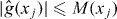
If we have a bound on the error of as an approximation to g, we can use it to check whether PAT has missed pieces of γg. For example, if we knew a function M(x) for which


it would suffice to evaluate g at grid points xj for which (perhaps starting with points for which is smallest) and check the sign of g at those points.
2.4.4. Random sampling and contour error.
We can use random sampling both to look for missing pieces and to collect statistical evidence about the accuracy of the PAT contour as an approximation to γg. Recall from section 1 that the difference between the true lower level set of g at level τ, Λτ, and the estimated lower level set of g, , is the set on which the approximate contour errs in classifying points in Δ. As discussed in the introduction, the approximate contour makes classification errors on two sets: points where the true value of g is strictly positive but the approximate contour claims that g is nonpositive, and points where the true value of g is nonpositive but the approximate contour claims that g is positive. The area of the union of those sets—the symmetric difference of Λτ and —is a measure of the accuracy of the approximate contour. Normalizing that area by the total area of Δ gives the fraction of the area of the domain Δ misclassified by the approximate contour.


To keep things simple, we consider how to estimate the fraction p of the area of Δ that is misclassified by the PAT contour —the relative area of the symmetric difference. The chance that a point selected at random uniformly from Δ is misclassified by is p. If a point near is misclassified, it could mean that is slightly out of place. If a point far from is misclassified, that suggests that is a missing piece of γg. To check, we can search for a root of g on any line segment between that point and the nearest piece of . If we find such a root, it becomes a starting point to trace a piece of γg that had been missed.


On the other hand, suppose we draw n points at random, independently, uniformly from Δ, and the sign of g at every point in the sample agrees with its sign according to the PAT contour : no point in the sample is in the symmetric difference . Then an event has occurred that has the probability (1 − p)n. We can use this to find a 1 − α upper confidence bound on p: for this event to have a probability greater than α, p must be less than 1 − α1/n. For instance, for n = 50, we would have 95% confidence that P < 5.8%; for n = 100, we would have 95% confidence that P < 3%.


More generally, if n independent draws find m misclassified points, a 1 − α upper confidence bound for the relative area of , the part of the domain Δ misclassified by the PAT contour, is


Evaluating g at a random sample of points in Δ allows us to have confidence in the accuracy of the PAT contour, despite the fact that the assumptions behind PAT might be wrong—at the expense of n extra evaluations of g.
In some applications, one kind of error is more important than the other. For instance, erroneously including extra points in a confidence set makes the set conservative, while erroneously excluding points from a confidence set is misleadingly optimistic. Moreover, the 'cost' of misclassifying points might be higher for some points than for others. For instance, erroneously excluding from a confidence set of climate models a model in which global temperature rises 10 K in 20 years might be a more serious error than erroneously excluding a model in which global temperature rises 0.5 K in 20 years. Such differences can be taken into account by using weighted areas (integration against a nonuniform measure instead of Lebesgue measure) and carrying out the above sampling using corresponding nonuniform distributions.
3. Tests of Pilot Approximation Trajectory
In this section we apply PAT to two test cases: finding a contour of a two-dimensional function with a saddle point, at the level of the saddle point, and constructing a confidence set in an inverse problem involving air flow.
3.1. Contouring a function with a saddle point
Let g be a sum of 2 two-dimensional Gaussian bumps:

where the matrices R and C and the vectors μ± are given by

The matrix R rotates the coordinate system 45° clockwise. The domain for the contour plot is Δ ≡ [ − 1,1]2. The function g is plotted in figure 4.

Figure 4. A function g with a saddle point used to test PAT and its pilot approximation .

Download figure:
Standard imageThis function has a saddle point at the origin. To test the ability of PAT to contour saddle points, we contour at level τ = g(0,0), the value of g at the saddle point.
The pilot approximation was chosen to be the piecewise linear approximation of g using an equispaced 9 × 9 grid in Δ (see description in section 1) and it is plotted in figure 4.

The PAT contour found using a 32 × 32 grid is plotted in figure 5. For comparison, figure 5 shows a contour computed using the built-in contouring algorithm in R with data on a 1024 × 1024 grid and on the 32 × 32 grid. The 1024 × 1024 grid is dense enough that the approximate contour is essentially the true contour of g. Figure 6 is a close-up of the contour near the saddle point.


Figure 5. Results for example 1: PAT contour of g (dots connected with black lines) and standard contour of (crosses connected with black lines) on a 32 × 32 grid. Contours of g and computed using a standard algorithm on a 1024 × 1024 grid are plotted as solid light gray curves. A standard contour on a 32 × 32 grid is plotted as dotted dark gray curves.


Download figure:
Standard image
Figure 6. Close-up of the contour near the saddle point (the origin). The approximate PAT contour of g is plotted as dots connected with black lines; the standard contour is plotted as a solid light gray line (1024 × 1024 grid) and a solid light gray line (32 × 32 grid).

Download figure:
Standard imageThe PAT contour is almost indistinguishable from the standard contour on a 1024 × 1024 grid. It is comparable to the standard contour on a 32 × 32 grid except near the saddle point, where the PAT contour is more accurate. PAT correctly finds that the contour crosses itself, even though the contour of the pilot approximation does not. Moreover, PAT is more accurate than the standard contouring algorithm on the 32 × 32 grid, in part because PAT locates zeros of g with a root finder rather than approximating them by linear interpolation. Indeed, if we treat the contour on the 1024 × 1024 grid as ground truth, the standard contouring on a 32 × 32 grid misclassifies 0.38% of the domain, while PAT misclassifies only 0.12% of the domain (the area of the symmetric difference was computed using the gpclib library in R. Repeated random samples of 100 points generally found none that were misclassified by the PAT contour (no sample point was in ). The 95% upper confidence bound on the fraction of Δ misclassified by the PAT contour based on a sample of size 100 that shows no misclassifications is about 3%, rather larger than the true percentage, 0.12%. Occasionally, a random sample of 100 points revealed one point misclassified by the PAT contour; the corresponding upper 95% confidence bound is 4.7%. By sampling more than 100 points, these upper confidence bounds could be reduced. However, the bounds decrease roughly like the reciprocal of the square root of the sample size. For instance, to reduce the 95% upper confidence bound from 3% to 0.2% would require evaluating g at least 1500 times, to reduce the sampling variability in the accuracy assessment—not to improve the contour.

To compute the PAT contour required evaluating g 370 times (the pilot approximation was evaluated 1109 times). To build the pilot approximation , g was evaluated 92 = 81 times, so g was evaluated 451 times in all. For comparison, computing the contour on a 32 × 32 grid using a standard contouring algorithm requires 322 = 1024 evaluations of g. In this example, our algorithm requires 56% fewer evaluations of g. Including the 100 evaluations of g at randomly selected points, the total number of evaluations is still 46% less than the standard contouring algorithm requires—and gives a more accurate contour and an internal measure of accuracy, which the standard method lacks. (Of course, the same sampling approach could be used to assess the accuracy of the standard method, at the cost of an additional 100 evaluations of g for parity.) The number of evaluations of g that PAT requires depends on the root-finding algorithm and its tuning constants; we used the algorithm of Müller (1956).


Missing contour pieces.
To test the ability of PAT to find a contour accurately even when the topology of the contour of the pilot approximation is wrong, we shifted the level τ for which the contour is constructed by 0.005 (i.e. τ = g(0,0) + 0.005). This makes the contour γg,τ consist of two closed curves. We also shifted the approximation by 0.045 so that the contour of the pilot approximation is a single closed curve that encircles both pieces of the contour γg,τ, so the contour γg,τ has more pieces than , the contour of the pilot approximation.


The method described in section 2.4 finds the piece. That method checks for whole-cell 'gaps' between the PAT contour and the approximate contour of the pilot approximation, . In this example, the missing piece of the PAT contour is inside the approximate contour, so the gaps are outside the PAT contour. Since g is below τ near but outside the PAT contour, the algorithm will detect that a piece of the contour is missing if it finds a point x outside the traced piece for which g(x) > τ. To look for such a point, it evaluates g within the gap at the grid point where is largest, since, if is a good approximation of g, we expect g to be large there, too. If g > τ at that point, the algorithm searches the line segment between that point and the closest point at which g has been already evaluated (a vertex of the cell intersected by the contour) to find a point where g = τ. It then traces the (new) piece of the contour that passes through that root of g − τ.


The PAT contour on a 32 × 32 grid is shown in figure 7. Computing the PAT contour required 423 evaluations of g: 82 = 64 to find the pilot approximation and 359 to trace the contour. If we consider the contour on the 1024 × 1024 grid to be the ground truth, the standard contour on a 32 × 32 grid misclassifies 0.33% of the domain, while PAT misclassifies only 0.15% of the domain. Again, PAT gives a more accurate contour than the standard method, using far fewer evaluations of g.

Figure 7. PAT contour for a shifted version of example 1. In this example, the true contour has two pieces but the contour of the pilot approximation has only one. The algorithm identifies the cells marked in black as a 'gap' between , the approximate contour of and , and the PAT contour of g. The black line segment joins the point at which is largest and the closest point in the gap at which g has already been evaluated. The algorithm searches that segment for a root of g − τ. The second piece of the PAT contour is traced starting at the root of g − τ on the black line segment. The solid and dotted gray curves are as described in figure 5.


Download figure:
Standard imageWorkload scaling.
To investigate empirically how the number of function evaluations PAT requires scales, we used PAT to contour the saddle function on grids ranging from 20 × 20 to 200 × 200. Table 1 gives the results. PAT's computational advantage over the standard method increases with the dimension of the grid. The number of evaluations of g for the standard method scales like the number of points in the grid, n2, while the number of evaluations of g for PAT scales approximately as O(n). The accuracy of PAT is substantially better than that of standard methods on coarse grids, and slightly better even for fine grids.
Table 1. Workload scaling for PAT and standard contouring for various grid dimensions, for the test function in figure 4. 'Saved' is 1 minus the ratio of evaluations of g for PAT to evaluations of g for the standard method. 'Relative error' is the ratio of the area of the symmetric difference of the true and approximate lower level sets for the standard contour to the area of that difference for the PAT contour. Numbers larger than 1.0 indicate that PAT is more accurate than the standard method.
| Grid dimension | Evaluations of g | Saved | Relative error | |
|---|---|---|---|---|
| PAT | Standard | |||
| 20×20 | 266+81 | 400 | 13% | 2.43 |
| 30×30 | 355+81 | 900 | 51% | 3.20 |
| 50×50 | 512+81 | 2500 | 76% | 1.49 |
| 100×100 | 910+81 | 10 000 | 90% | 1.07 |
| 200×200 | 1814+81 | 40 000 | 95% | 1.06 |
4. Test case 2: confidence sets for viscosity and thermal conductivity of airflow
An ideal homogeneous gas flows from left to right in a two-dimensional pipe, sketched in figure 8. The gas is heated at the input boundary on the left with a known temperature profile. There is no heat source within the pipe. Once the flow is in a steady state, the temperature of the gas is measured at 101 points shown in figure 8; the measurements have iid additive Gaussian noise with an expected value of 0 and variance of 1. From the boundary condition and the temperature measurements, we want to estimate the viscosity and the thermal conductivity of the gas and to find the uncertainties of the estimates using a confidence set, as described in the appendix.

Figure 8. The computational domain for the gas flow example, a two-dimensional pipe whose diameter doubles abruptly. An ideal gas flows in through Γin on the left and out through Γout on the right. The inner wall of the pipe is the boundary Γwall (not labeled). Boundary conditions are imposed on temperature and velocity at Γin, there is no flow across the pipe wall and the velocity through Γout is purely horizontal. Steady-state temperature is measured with independent, additive, zero-mean Gaussian noise at the 101 points indicated by crosses.
Download figure:
Standard imageWe model the flow using Elmer finite-element software (IT Center for Science (CSC) 2011). The diameter of the pipe has a step, which causes the flow to detach from the wall. If the viscosity is sufficiently small (i.e., if the Reynolds number is large), the flow may become turbulent, a possibility we ignore in this example.
Mathematical models.
The steady-state temperature distribution T(·) of the gas is modeled by the heat equation. Since there are no internal sources, this equation is:

where C is heat capacity, v is the velocity field and κ is thermal conductivity. The velocity field is modeled by the Navier–Stokes equation:

where ρ is density, μ is viscosity, p is pressure, h is gravitational force and is the infinitesimal strain tensor. The velocity and temperature boundary conditions at the input boundary vary quadratically with height. The velocities at the walls are zero and purely horizontal at the output boundary. The temperature at the walls is fixed, and the flow satisfies the Neumann zero boundary condition at Γout.
We solved the heat equation and the Navier–Stokes equation as coupled PDEs using Elmer. The function f and its pilot approximation (see the notation in the appendix) are as follows. The function f maps (x1,x2) to HT, where T is the temperature distribution for a fixed viscosity of 10−x1 Ns m−2 and a fixed thermal conductivity of 10−2·x2 W (m K)−1, and H is the matrix that interpolates linearly between points on the computational mesh to calculate T at the measurement points. The domain of f is Δ = [3,4] × [2,3], which we verified experimentally to contain every point in the confidence set. A logarithmic transformation of viscosity improves numerical stability, since the effect of viscosity on velocity and temperature is exponential. We scaled the x2-axis to make the axes equally long to improve computational efficiency. An approximation for f is formed in the same way using a very sparse mesh.


Results.
We used PAT to approximate the contour corresponding to the boundary of the 95% χ2 confidence set (see the appendix). The function g was defined using (A.2) with p = 2 (χ2 confidence sets). The pilot approximation is obtained similarly by replacing f with in equation (A.2).


The computational mesh used to evaluate f contained 330 elements and 1099 nodes. For the pilot approximation , the mesh contained 108 elements and 389 nodes. Elmer becomes unstable in this problem if there are significantly fewer elements than that. The material parameters used in the computations are shown in table 2. PAT contours were computed using a grid of 30 × 30 cells (31 × 31 grid points).

Table 2. Material properties for gas-flow simulations.
| Parameter | Value |
|---|---|
| Viscosity | 1/5500 Ns m−2 |
| Thermal conductivity κ | 2.55×10⁻² W (m K)−1 |
| Heat capacity C | 1010 J (kg K)−1 |
| Specific heat ratio | 1.4 |
| Reference pressure | 105 Pa |
The simulated data were computed using Elmer with a dense mesh of 563 elements and 1830 nodes. Independent, identically distributed zero-mean Gaussian noise with standard deviation 2.79 K (2% of the elevation in the temperature) was added to the simulated values.
To assess accuracy of the PAT confidence sets, we also computed the contour using the standard algorithm in R on a 256 × 256 grid. The PAT contours and reference contours are shown in figure 9. The PAT contours are almost indistinguishable from contours computed by standard methods on the dense grid. Differences are visible only in sharp corners where the cell size is too large for a straight line segment to turn as rapidly as the actual contour.

Figure 9. The χ2 confidence set. The black dots connected with lines are the PAT contour of the actual misfit function. The crosses are the contour of the pilot approximation for PAT. The solid gray lines are contours computed using a standard algorithm on a 256 × 256 grid.
Download figure:
Standard imageComputing the PAT contour for the χ2 confidence set required evaluating the function f 243 times and the function 1023 times. The number of the evaluations of f was about a quarter of 312 = 961, the minimum number of evaluations a standard contouring method would use to compute the contour on a 31 × 31 grid. Moreover, the PAT contour is more accurate than the standard contouring method on a 31 × 31 grid: the relative area of for the PAT confidence set is 0.06% while the relative area for a standard contour on the same grid is 0.15%.


5. Conclusions
The PAT algorithm can find one or more contours of a function g using fewer evaluations of g than traditional contouring methods, which can entail substantial savings if g is expensive to evaluate. PAT uses an inexpensive pilot approximation of g to predict the location of the contour. This can reduce the number of evaluations of g required to contour g to a given level of accuracy. PAT uses an iterative method to find points on the contour, and takes advantage of the fact that g can be evaluated anywhere, not just on the vertices of a regular grid.
The computational advantage of PAT increases with the dimension of the grid used in the standard method. In examples, the number of function evaluations that PAT requires scales roughly as the square root of the number of grid points, while conventional methods scale linearly with the number of grid points. The savings can be enormous. In our experience, changing the accuracy of the pilot approximation does not affect the workload much unless it changes the number of disjointed pieces that the contour of the pilot approximation has.
Two numerical examples illustrate the utility and efficiency of PAT. The first example is to contour a function that has a saddle point near the contour level. The second example is to find a χ2 confidence set for an unknown two-dimensional parameter in a nonlinear inverse problem. In both examples, PAT contours are more accurate than standard contours and require only a fraction as many function evaluations. PAT is particularly useful to contour functions that are expensive to evaluate, for example, when evaluating the function requires conducting a physical experiment or running complex coupled PDE solvers.
Since PAT uses values of g at cell vertices to determine whether the contour crosses an edge, PAT cannot tell whether an edge is intersected more than once. Reducing cell size ameliorates this issue, but increases the number of evaluations of g. A more sophisticated approach might split cells adaptively depending on the local smoothness of g. Aramini (1980) proposes adapting grid size locally using the Laplacian of g or the value of g at the centers of cells. Similar techniques might be used with PAT. For PAT, a criterion for splitting cells might be based on (e.g., tracing the contour of on a dense grid to see whether it crosses any edge more than once).


As presented here, PAT is for functions of two variables. PAT could be extended to functions of three variables using an approach similar to Marching cubes (Lorensen and Cline 1987; see also Bhaniramka et al 2004, Schreiner et al 2006). How to extend PAT to dimensions higher than three is an open question.
Acknowledgments
JMJH was supported by the Osk. Huttunen Foundation, the Jenny & Artturi Wihuri Foundation and the Finnish Cultural Foundation, and the Academy of Finland (application number 213476, the Finnish Programme for Centres of Excellence in Research 2006–2011). PBS received support from Lawrence Livermore National Laboratory grant B585264.
Appendix.: Confidence sets based on χ2 misfit
This section sketches a standard approach to constructing a confidence set for a collection of parameters in an inverse problem. The approach, sometimes called strict bounds, is not optimal but it is conservative. For more detail, see, for instance, Evans and Stark (2002).
Consider estimating the parameter from observations that are related through


where f is a known function, is stochastic observational error and x0 is an unknown element of the measurable set .

The function f maps into an n-vector (f1(x),...,fn(x))T. Computing f might involve Monte Carlo simulation or the numerical solution of a PDE by finite-element methods, but we ignore uncertainty in calculating f(x0) for known x0. See Stark (1992, 2008) or Kaipio and Somersalo (2005) for a treatment of systematic errors in inverse problems, such as errors that result from approximating f.

The additive error is a random n-vector (1,...,n)T. The error has an expected value of zero and known, finite, positive-definite covariance matrix . Let be the standard deviation of the kth component of . The parameter x0 is fixed; the only random element in the problem is the error .


Suppose C(·) is a measurable mapping from the data space into subsets of the parameter space . If C satisfies


then C is a 1 − α confidence procedure. Inequality (A.1) says that the coverage probability of C(Y ) is at least 1 − α, whatever be . If we observe the datum Y =y, then C(y) is a 1 − α confidence set for x0.

Before the data are observed, C(Y ) is not a fixed set—it is random—and it is meaningful to talk about the chance that C(Y ) will end up containing x0. In repeated experiments, the fraction of 95% confidence sets that include the true parameter value x0 converges in probability to 95%, by the Law of Large Numbers. Once the data have been observed, we talk about confidence level rather than coverage probability: nothing random is left. For instance, the assertion

does not make sense because x0 is a fixed parameter and C(y) is a fixed set. Either x0 is in C(y) or not; there is no probability.
We consider confidence sets derived from misfit functions: the confidence set contains all parameter values for which the predicted data agree adequately with the observed data. Agreement is measured in a norm. 'Adequately' is calibrated to make the coverage probability 1 − α.
Let ∥·∥p,Σ be a p-norm on with weights derived from Σ.

For instance, for p = 2 we might define
or, for p = ∞,

Let χp,Σ,α be the smallest value of c for which
Then

So, if we define

then C(Y ) is a 1 − α confidence set for x0; see, for instance, Stark (1992) for examples and extensions. The case p = 2 is sometimes called a χ2 confidence set; the case p = ∞ is sometimes called a maximum modulus confidence set.
As a concrete example, suppose the n components of are independent, iid zero-mean Gaussian random variables with common variance σ2. Then Σ = σ2I, where I is the n by n identity matrix; χ2,Σ,α is σ times the square root of the 1 − α percentage point of the χ2 distribution with n degrees of freedom.
For a fixed choice of p and α and a fixed y, define the real-valued function g on :


A 1 − α confidence set for x0 based on the observation Y =y is thus

This is the lower level set of g at level τ = 0. Continuity of g follows from continuity of the p-norm and the assumed continuity of f. Hence, the confidence set—which typically is not simply connected—is closed relative to , and the contour γg,0 = {x:g(x) = 0} is the boundary of the confidence set.

Footnotes
- 4
We do not address how to select the appropriate cell size, but the pilot approximation may be helpful. See, e.g., Aramini (1980) for methods of selecting cell size.
