
Abstract
The notion of random motion in a potential well is elemental in the physical sciences and beyond. Quantitatively, this notion is described by reverting diffusions—asymptotically stationary diffusion processes which are simultaneously (i) driven toward a reversion level by a deterministic force, and (ii) perturbed off the reversion level by a random white noise. The archetypal example of reverting diffusions is the Ornstein–Uhlenbeck process, which is mean-reverting. In this paper we analyze reverting diffusions and establish that: (i) if the magnitude of the perturbing noise is constant then the diffusion's stationary density is unimodal and the diffusion is mode-reverting; (ii) if the magnitude of the perturbing noise is non-constant then, in general, neither is the diffusion's stationary density unimodal, nor is the diffusion mode-reverting. In the latter case we further establish a result asserting when unimodality and mode-reversion do hold. In particular, we demonstrate that the notion of mean-reversion, which is fundamental in economics and finance, is a misconception—as mean-reversion is an exception rather than the norm.
Export citation and abstract BibTeX RIS
1. Introduction
Mean-reversion is a fundamental concept in economics and finance proposing that, over time, prices and indices revert to their historical means [1–5]. Quantitatively, mean-reversion is modeled by the Ornstein–Uhlenbeck process, whose stochastic dynamics are given by

In equation (1) (X(t))t ⩾ 0 is the Ornstein–Uhlenbeck process under consideration, l is the level toward which the process reverts (l real), r is the relaxation rate of the reversion (r positive), σ is the magnitude of the perturbing noise (σ positive), and  is the perturbing noise—the temporal derivative of the Wiener process (W(t))t ⩾ 0 (Brownian motion).
Equation (1)—governing the stochastic dynamics of the Ornstein–Uhlenbeck process—is one of the most elemental stochastic differential equations in science and engineering [6–8]. Stochastic differential equations play a predominant role, if not to say a focal role, in continuous-time financial models [9]: 'Continuous-time modeling in finance, though introduced by Louis Bachelier's 1900 thesis on the theory of speculation [10], really started with Merton's seminal work in the 1970s [11]. Since then, the continuous-time paradigm has proved to be an immensely useful tool in finance and more generally economics.' Throughout this paper we shall follow the financial-economic paradigm [12] of interpreting stochastic differential equations via the Ito calculus [13]—rather than via the Stratonovich calculus [14] (which is often applied in the physical sciences).
The Ornstein–Uhlenbeck process was introduced and pioneered by Uhlenbeck and Ornstein [15], and has a wide spectrum of applications ranging from physics to biology, and from engineering to economics [16, 17]. From a physical-sciences perspective the Ornstein–Uhlenbeck process models the motion of a particle trapped in a harmonic potential well and perturbed by random thermal fluctuations [16, 17]. One of the most popular applications of the Ornstein–Uhlenbeck process in finance is the Vasicek model for spot interest rates [18, 19]. In the recent years the Ornstein–Uhlenbeck process has attracted significant interest in the context of anomalous diffusion [20–28].
The Ornstein–Uhlenbeck process is a special case of reverting diffusions—asymptotically stationary diffusion processes which are simultaneously and continuously (i) subject to a deterministic restoring force which drives them toward a reversion level l, and (ii) perturbed by a random white noise which drives them off the reversion level l. A reverting diffusion process converges in law (as t → ∞) to a stochastic steady state. This steady state manifests the 'stochastic balance' between the diffusion's opposing drivers—the deterministic restoring force and the random perturbing white noise. The stationary distribution governing the steady state of the Ornstein–Uhlenbeck process is Gaussian with mean l and variance σ2/2r, and its probability density function is given by

(−∞ < x < ∞; cG being a normalizing constant). The Gaussian density ϕG(x) is the stationary solution of the Fokker–Planck equation corresponding to the stochastic dynamics of equation (1) [29].
The Ornstein–Uhlenbeck restoring force is quantified by the function F(x) = r(x − l). This function is negative valued for x < l, and is positive valued for x > l. Thus, the Ornstein–Uhlenbeck restoring force indeed reverts the process (X(t))t ⩾ 0 toward the reversion level l. On the other hand, the level l is the mean of the Ornstein–Uhlenbeck stationary distribution. Moreover, the Ornstein–Uhlenbeck stationary density ϕG(x) is unimodal and it attains its mode at the level l. Hence, the Ornstein–Uhlenbeck process is both mean-reverting and mode-reverting.
Mean-reversion is a rather particular behavior displayed by the Ornstein–Uhlenbeck process—which is a very specific reverting diffusion characterized by a linear restoring force (F(x) = r(x − l)), and by a constant noise magnitude (σ). The goal of this paper is to demonstrate that the concept of mean-reversion is, in effect, a misconception—as mean-reversion is an exception rather than the norm. In this paper we analyze general reverting diffusions and establish that:
- If the magnitude of the diffusion's perturbing white noise is constant then the diffusion's stationary density is always unimodal, and the diffusion is always mode-reverting.
- If the magnitude of the diffusion's perturbing white noise is non-constant then, in general, the diffusion's stationary density is not necessarily unimodal, and the diffusion is not necessarily mode-reverting.
In the former case of constant noise magnitudes—which is studied in section 2—we provide examples illustrating the failure of mean-reversion. In the latter case of non-constant noise magnitudes—which is studied in section 3—we further establish a general result asserting when unimodality and mode-reversion do hold, and we provide an array of examples illustrating the diversity of 'non mode-reversion' scenarios that can take place.
2. Langevin dynamics
In this section we study the case of reverting diffusions with constant noise magnitudes.
2.1. Analysis of Langevin dynamics
As noted in the introduction the Ornstein–Uhlenbeck restoring force is quantified by the function F(x) = r(x − l). This force function is linear, and is thus rather particular and specific. If we replace the linear Ornstein–Uhlenbeck force function by a nonlinear force function we arrive at the Langevin stochastic differential equation

The Langevin equation (3) was introduced and pioneered by Paul Langevin [30], and is a cornerstone equation in the physical sciences [31–35].
As in the case of the Ornstein–Uhlenbeck process we consider the Langevin force function F(x) to be reverting toward a reversion level l. Namely, we consider the Langevin force function F(x) to be negative valued for x < l, and to be positive valued for x > l. The random process (X(t))t ⩾ 0 governed by the Langevin equation (3) is asymptotically stationary, and it converges in law (as t → ∞) to a stochastic steady state which manifests the 'stochastic balance' between the two opposing drivers—the Langevin restoring force and the perturbing white noise. The stationary distribution governing the steady state of the Langevin equation (3) is quantified by the probability density function

(−∞ < x < ∞; cL being a normalizing constant). The density ϕL(x) is the stationary solution of the Fokker–Planck equation corresponding to the Langevin equation (3) [29]. The necessary and sufficient condition required to assure the validity of equation (4) is the integrability of the density ϕL(x) over the real line. The function V(x) = ∫xF(s)ds (−∞ < x < ∞) appearing in equation (4) is a potential corresponding to the Langevin force function F(x).
The shape of the Langevin force function F(x)—negative valued below the reversion level, and positive valued above the reversion level—straightforwardly implies that the density ϕL(x) is unimodal, and that it attains its global maximum at the level l. Namely, the reversion level l is the mode of the density ϕL(x)—the stationary density of the Langevin dynamics. Thus, shifting from a linear Ornstein–Uhlenbeck restoring force to a nonlinear Langevin restoring force we conclude that:
- Mode-reversion always holds but, in general, mean-reversion is not bound to hold.
- In the special case where the Langevin stationary density is symmetric around its mode, and possesses a well-defined mean, then the mode and the mean coincide, and the reversion is to the common mode-mean.
In the case of the Ornstein–Uhlenbeck process the stationary distribution is Gaussian. The Gaussian distribution has finite moments, and its density is unimodal and is symmetric around its mode. Hence, the mean of the Gaussian distribution is well defined, and it coincides with the Gaussian mode. In contrast, in the case of general Langevin dynamics neither must the mean be well defined, nor does it necessarily coincide with the mode.
2.2. Examples of Langevin dynamics
The following examples illustrate the 'failure of mean-reversion' in the context of Langevin dynamics. In all the examples we set, with no loss of generality,  .
.
Laplace example. Consider the nonlinear force function given by: F(x) = −p− for x < 0, and F(x) = p+ for x > 0 (where p− and p+ are positive parameters). The reversion level of this force function is the origin l = 0, and the resulting stationary density is Laplace: ϕL(x) = cLexp ( − p−|x|) for x < 0, and ϕL(x) = cLexp ( − p+|x|) for x > 0. This Laplace density is unimodal, it attains its mode at the origin, and it is symmetric around its mode if and only if p− = p+. The mean of this Laplace density is (1/p+) − (1/p−). Thus, mean-reversion holds only in the symmetric scenario characterized by p− = p+.
Student example. Consider the nonlinear force function F(x) = (1 + p)x/(p + x2) (where p is a positive parameter). The reversion level of this force function is the origin l = 0, and the resulting stationary density is Student: ϕL(x) = cL/(1 + x2/p)(1 + p)/2. The parameter value p = 1 yields a Cauchy–Lorentz density, and the parameter limit p → ∞ yields a Gauss density. This Student density is unimodal, it attains its mode at the origin, and it is symmetric around its mode. The mean of this Student density is ill-defined in the parameter range p ⩽ 1, and is zero in the parameter range p > 1. Thus, although this Student density is symmetric around its mode—the very notion of mean-reversion is well-defined only in the parameter range p > 1.
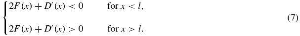
Gamma example. In this example the Langevin dynamics take place on the positive half-line (x > 0). Consider the nonlinear force function F(x) = 1 − p/x (where p is a positive parameter). The reversion level of this force function is l = p, and the resulting stationary density is Gamma: ϕL(x) = cLexp ( − x)xp (x > 0). This Gamma density is unimodal and skewed, and it attains its mode at the reversion level l = p. The mean of this Gamma density is p + 1. Thus, the mean is always greater than the mode—implying that mean-reversion never holds. This example is schematically illustrated in figure 1.

Figure 1. Gamma distribution via Langevin dynamics. The dynamics take place on the positive half-line (x > 0), the reversion level is ℓ = 2, the magnitude of the perturbing noise is  , the force function is
  (solid curve), and the resulting stationary density is Gamma:
  exp ( − x)x2 (dashed curve). The mode is 2 and the dynamics are mode-reverting. The mean is 3 and the dynamics are not mean-reverting.
Download figure:
Standard imageInverse Gamma example. In this example the Langevin dynamics take place on the positive half-line (x > 0). Consider the nonlinear force function F(x) = (p + 1 − 1/x)/x (where p is a positive parameter). The reversion level of this force function is l = 1/(p + 1), and the resulting stationary density is inverse Gamma: ϕL(x) = cLexp ( − 1/x)/xp + 1 (x > 0). This inverse Gamma density is unimodal and skewed, and it attains its mode at the reversion level l = 1/(p + 1). The mean of this inverse Gamma density is infinite in the parameter range p ⩽ 1, and is given by 1/(p − 1) in the parameter range p > 1. Thus, the mean is always greater than the mode—implying that mean-reversion never holds.
Pareto example. In this example the Langevin dynamics take place on the positive half-line (x > 0). Consider the nonlinear force function F(x) = (1 + p)/(1 + x) (where p is a positive parameter). The reversion level of this force function is the origin l = 0, and the resulting stationary density is Pareto: ϕL(x) = cL/(1 + x)1 + p (x > 0). This Pareto density is monotone decreasing, and it attains its mode at the reversion level l = 0. The mean of this Pareto density is infinite in the parameter range p ⩽ 1, and is given by 1/(p − 1) in the parameter range p > 1. Thus, the mean is always greater than the mode—implying that mean-reversion never holds. This example—in the parameter range p > 1—is schematically illustrated in figure 2.

Figure 2. Pareto distribution via Langevin dynamics. The dynamics take place on the positive half-line (x > 0), the reversion level is the origin ℓ = 0 , the magnitude of the perturbing noise is  , the force function is
  (solid curve), and the resulting stationary density is Pareto:
  (dashed curve). The mode is 0 and the dynamics are mode-reverting. The mean is 1 and the dynamics are not mean-reverting.
Download figure:
Standard imageWe note that the Student example, the inverse Gamma example, and the Pareto example represent scenarios of Langevin dynamics taking place in asymptotically logarithmic potential wells—which are of significant importance in statistical physics [36, 37].
3. Diffusion dynamics
In this section we study the case of reverting diffusions with non-constant noise magnitudes.
3.1. Analysis of diffusion dynamics
The stochastic dynamics governing the Ornstein–Uhlenbeck process are a sub-class of the more general Langevin dynamics. In turn, the Langevin dynamics are a sub-class of general diffusion dynamics given by the stochastic differential equation

In equation (5) the magnitude of the perturbing noise is state-dependent and is quantified by the diffusion function D(x)—a positive valued and smooth function defined on the real line. Namely, when the process (X(t))t ⩾ 0 is at the state x then the magnitude of the perturbing noise is  . The special case of Langevin dynamics is characterized by constant diffusion functions: D(x) ≡ σ2.
The predominate and focal role of general diffusion dynamics in continuous-time financial models is eloquently pinpointed in [9]: 'Continuous-time models are widely used to study issues that include the decision to optimally consume, save, and invest, portfolio choice under a variety of constraints, contingent claim pricing, capital accumulation, resource extraction, game theory, and more recently contract theory. Many refinements and extensions are possible, but the basic dynamic model for the variable(s) of interest X(t)is a stochastic differential equation (of the form given by equation (5))'. Equation (5) is indeed the very bedrock of contemporary continuous-time financial models [19, 38–40].
As in the case of the Ornstein–Uhlenbeck process, and as in the case of Langevin dynamics, we consider the force function F(x) to be pushing toward a reversion level l. Namely, we consider the force function F(x) to be negative valued for x < l, and to be positive valued for x > l. The random process (X(t))t ⩾ 0 governed by the stochastic differential equation (5) is asymptotically stationary, and it converges in law (as t → ∞) to a stochastic steady state which manifests the 'stochastic balance' between the two opposing drivers—the restoring force and the perturbing white noise. The stationary distribution governing the steady state of the random process (X(t))t ⩾ 0 is quantified by the probability density function

(−∞ < x < ∞; cD being a normalizing constant). The density ϕD(x) is the stationary solution of the Fokker–Planck equation corresponding to the stochastic differential equation (5) [29]. The necessary and sufficient condition required to assure the validity of equation (6) is the integrability of the density ϕD(x) over the real line.
A straightforward analysis applied to the stationary density ϕD(x) yields the following mode-reversion and mean-reversion conclusions:
- The stationary density ϕD(x) is unimodal, and its mode coincides with the reversion level l, if and only if the following condition holds:

- If—in addition to the condition of equation (7)—the stationary density ϕD(x) is symmetric around its mode, and possesses a well-defined mean, then the mode and the mean coincide, and the reversion is to the common mode-mean.
Note that in the case of Langevin dynamics D'(x) ≡ 0 and hence the condition of equation (7) is trivially satisfied. In the physical sciences scenarios involving potential functions with multiple minima are prevalent. A potential function V(x) induces the force function F(x) = V'(x), and a natural question arising is: do the minima of the potential function V(x) coincide with the modes of the corresponding stationary densityϕD(x)? Consider a potential function V(x) with extrema attained at the points l1 < l2 < ⋅⋅⋅ < ln, where: n is an odd integer, the oddly indexed extremal points are local minima, and the evenly indexed extremal points are local maxima. This implies that the force function F(x) is negative valued on the intervals {( − ∞, l1), (l2, l3), ...(ln − 1, ln)}, and is positive valued on the intervals {(l1, l2), (l3, l4), ...(ln, ∞)}. The shape of the potential function V(x) is reflected in the shape of the stationary density ϕD(x) if and only if the extrema of both these functions coincide, and the oddly indexed extremal points are local maxima of ϕD(x), and the evenly indexed extremal points are local minima of ϕD(x). A straightforward analysis of the stationary density ϕD(x) implies that 'shape reflection' holds if and only if the function 2F(x) + D'(x) is negative valued on the intervals {( − ∞, l1), (l2, l3), ...(ln − 1, ln)}, and is positive valued on the intervals {(l1, l2), (l3, l4), ...(ln, ∞)}. This conclusion is the multimodal analogue of the unimodal mode-reversion conclusion stated above. As in the unimodal setting—in the case of Langevin dynamics D'(x) ≡ 0 and hence 'shape reflection' always holds.
3.2. Transformations of the Ornstein–Uhlenbeck process
In this subsection we consider two transformations of the Ornstein–Uhlenbeck process. These transformations exemplify—even in the context of the mean-reverting Ornstein–Uhlenbeck process—how non-constant diffusion functions naturally arise, and how both mode-reversion and mean-reversion can fail to hold. Throughout this subsection (X(t))t ⩾ 0 denotes the Ornstein–Uhlenbeck process presented in the introduction.
The first transformation considers the square displacement of the Ornstein–Uhlenbeck process off its mean, i.e. the process (X1(t))t ⩾ 0 given by X1(t) = (X(t) − l)2. The square-displacement process (X1(t))t ⩾ 0 is non-negative valued. Moreover, Ito's formula [13] implies that the stochastic dynamics of the square-displacement process (X1(t))t ⩾ 0 are governed by the diffusion dynamics of equation (5), with force function F1(x) = 2rx − σ2 (x ⩾ 0), and with diffusion function D1(x) = 4σ2x (x ⩾ 0). The reversion level of this force function is l1 = σ2/(2r). Plugging these force and diffusion functions into equation (6) yields the Gamma density

(x > 0). This Gamma density is monotone decreasing, and its mode is attained at the origin (yielding an infinite peak). Moreover, the mean of this Gamma density is well-defined and is σ2/(2r). Hence, the reversion level coincides with the mean and is greater than the mode: mode < mean =l1. We conclude that when passing from the Ornstein–Uhlenbeck process (X(t))t ⩾ 0 to the square-displacement process (X1(t))t ⩾ 0 we lose the mode-reversion, but yet we retain the mean-reversion.
The second transformation considers the exponentiation of the Ornstein–Uhlenbeck process, i.e. the process (X2(t))t ⩾ 0 given by X2(t) = exp (X(t)). Exponentiation is commonplace in settings where the dynamics are multiplicative (rather than additive), and where temporal changes are measured in percentages; such settings are widespread in economics and finance [19, 41], and appear also in the physical sciences—e.g., [42–44]. The geometric Ornstein–Uhlenbeck process (X2(t))t ⩾ 0 is positive valued. Moreover, Ito's formula [13] implies that the stochastic dynamics of the geometric Ornstein–Uhlenbeck process (X2(t))t ⩾ 0 are governed by the diffusion dynamics of equation (5), with force function F2(x) = x[r(ln (x) − l) − σ2/2] (x > 0), and with diffusion function D2(x) = σ2x2 (x > 0). The reversion level of this force function is l2 = exp (l + σ2/(2r)). Plugging these force and diffusion functions into equation (6) yields the lognormal density

(x > 0). This lognormal density is unimodal and skewed, and it attains its mode at the level exp (l − σ2/(2r)). Moreover, the mean of this lognormal density is well-defined and is exp (l + σ2/(4r)). Hence, the reversion level is greater than the mean, and the mean is greater than the mode: mode < mean<l2. We conclude that when passing from the Ornstein–Uhlenbeck process (X(t))t ⩾ 0 to the geometric Ornstein–Uhlenbeck process (X2(t))t ⩾ 0 we lose both the mode-reversion and the mean-reversion.
3.3. Examples of diffusion dynamics
The following examples demonstrate the wide range of behaviors that emerge once the diffusion functions are non-constant.
Logistic example. Consider the hyperbolic-sine force function F(x) = (p/2)sinh (x) (where p is a positive parameter), and the hyperbolic-cosine diffusion function D(x) = cosh (x). The reversion level of this force function is the origin l = 0, and the resulting stationary density is logistic: ϕD(x) = cD(cosh (x))−p − 1. This logistic density is unimodal, it attains its mode at the origin, and it is symmetric around its mode. The mean of this logistic density is zero. Thus, the reversion level l coincides with both the mode and the mean, and we have reversion to the common mode-mean. Note that in this example the condition of equation (7) is indeed satisfied.
Student example. Consider the force function  , and the diffusion function
  (where p is a positive parameter). The reversion level of this force function is the origin l = 0, and the resulting stationary density is Student: ϕD(x) = cD/(1 + x2/p)(1 + p)/2. This Student density is unimodal, it attains its mode at the origin, and it is symmetric around its mode. The mean of this Student density is ill-defined in the parameter range p ⩽ 1, and is zero in the parameter range p > 1. Thus, the very notion of mean-reversion is well-defined only in the parameter range p > 1; in this parameter range the reversion level l coincides with both the mode and the mean, and we have reversion to the common mode-mean. Note that in this example the condition of equation (7) is indeed satisfied.
Gamma example. In this example the diffusion dynamics take place on the positive half-line (x > 0). Consider the linear force function F(x) = (x − p)/2 (where p is a positive parameter), and the linear diffusion function D(x) = x. The reversion level of this force function is l = p, and the resulting stationary density is Gamma: ϕD(x) = cDexp ( − x)xp − 1 ( x > 0). In the parameter range p ⩽ 1 this Gamma density is monotone decreasing, and its mode is attained at the origin (yielding an infinite peak). In the parameter range p > 1 this Gamma density is unimodal and skewed, and it attains its mode at the level p − 1. The mean of this Gamma density is p. Thus, the reversion level coincides with the mean and is greater than the mode: mode < mean =l. Namely, in this example mean-reversion always holds, whereas mode-reversion never holds. This example—in the parameter range p > 1—is schematically illustrated in figure 3.
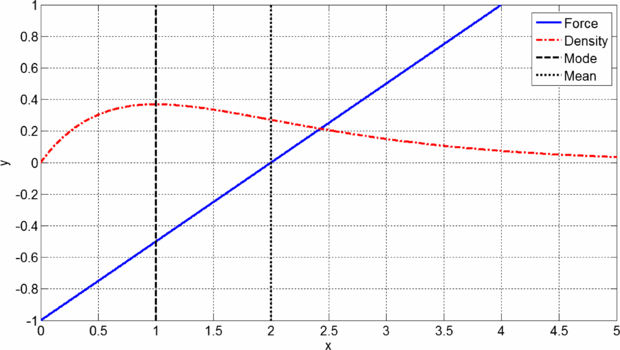
Figure 3. Gamma distribution via diffusion dynamics. The dynamics take place on the positive half-line (x > 0), the reversion level is ℓ = 2, the force function is  (solid curve), the diffusion function is D(x) = x, and the resulting stationary density is Gamma: ϕL(x) = exp ( − x)x (dashed curve). The mode is 1 and the dynamics are not mode-reverting. The mean is 2 and the dynamics are mean-reverting.
Download figure:
Standard imageInverse Gamma example. In this example the diffusion dynamics take place on the positive half-line (x > 0). Consider the force function F(x) = (p − 1/x)/2 (where p is a positive parameter), and the linear diffusion function D(x) = x. The reversion level of this force function is l = 1/p, and the resulting stationary density is inverse Gamma: ϕD(x) = cDexp ( − 1/x)/xp + 1 (x > 0). This inverse Gamma density is unimodal and skewed, and it attains its mode at the level 1/(p + 1). The mean of this inverse Gamma density is infinite in the parameter range p ⩽ 1, and is given by 1/(p − 1) in the parameter range p > 1. Thus, the reversion level is greater than the mode and is smaller than the mean: mode <l < mean. Namely, in this example neither mode-reversion nor mean-reversion ever hold.
Pareto example. In this example the diffusion dynamics take place on the positive half-line (x > 0). Consider the constant force function F(x) = p/2 (where p is a positive parameter), and the linear diffusion function D(x) = 1 + x. The reversion level of this force function is l = 0, and the resulting stationary density is Pareto: ϕD(x) = cD/(1 + x)1 + p (x > 0). This Pareto density is monotone decreasing, and it attains its mode at the reversion level l = 0. The mean of this Pareto density is infinite in the parameter range p ⩽ 1, and is given by 1/(p − 1) in the parameter range p > 1. Thus, the reversion level coincides with the mode and is smaller than the mean: l =mode < mean. Namely, in this example mode-reversion always holds, whereas mean-reversion never holds. Note that in this example the condition of equation (7) is indeed satisfied. This example—in the parameter range p > 1—is schematically illustrated in figure 4.
Figure 4. Pareto distribution via diffusion dynamics. The dynamics take place on the positive half-line (x > 0), the reversion level is the origin ℓ = 0, the force function is constant F(x) = 1 (solid curve), the diffusion function is D(x) = 1 + x, and the resulting stationary density is Pareto:  (dashed curve). The mode is 0 and the dynamics are mode-reverting. The mean is 1 and the dynamics are not mean-reverting.
Download figure:
Standard imageA class of examples. Consider a diffusion function D(x) which is symmetric around the origin, and a force function given by F(x) = −(p−/2)D(x) for x < 0, and given by F(x) = (p+/2)D(x) for x > 0 (where p− and p+ are positive constants). The reversion level of this force function is the origin l = 0, and the resulting stationary density is
This density is unimodal if and only if the function 1/D(x) is non increasing on the positive half-line (x > 0)—in which case the mode of the density is attained at the origin, and mode-reversion holds. On the other hand, this density is symmetric around the origin if and only if p− = p+—in which case its mean is zero, provided that its mean is indeed well defined. In what follows we show how different choices of the diffusion function D(x), and of the parameters p− and p+, can yield very different examples.
Example I: D(x) = 1/|x|. In this example the density ϕD(x) is bi-modal: it has a local maximum at the level −1/p−, has a global minimum at the origin, and has a local maximum at the level 1/p+. Moreover, the mean of this density is well-defined. Hence, in this example: (i) the reversion is to the most improbable value of the density; (ii) the notion of mode-reversion is ill-defined—since the density is not unimodal; (iii) mean-reversion holds if and only if p− = p+.
Example II:  , and p− = p+ = 1. In this example the density ϕD(x) is bi-modal: it attains its global maxima at the levels ±1, and it attains its global minimum at the origin. However, this density has no well-defined mean. Hence, in this example: (i) the reversion is to the most improbable value of the density; (ii) the notion of mode-reversion is ill-defined—since the density is not unimodal; (iii) the notion of mean-reversion is ill-defined—since the density does not have a well-defined mean.
Example III: D(x) = 1/(2 + cos (x)). In this example the density ϕD(x) is infinite-modal: it has infinitely many local minima and local maxima, and it attains its global maximum at the origin. Moreover, the mean of this density is well-defined. Hence, in this example: (i) the reversion is to the most probable value of the density; (ii) the notion of mode-reversion is ill-defined—since the density is not unimodal; (iii) mean-reversion holds if and only if p− = p+.
Example IV: D(x) = 1/(sin (x))2. In this example the density ϕD(x) is infinite-modal: it has infinitely many local maxima, and infinitely many global minima—one of them attained at the origin. Moreover, the mean of this density is well-defined. Hence, in this example: (i) the reversion is to one of the most improbable values of the density; (ii) the notion of mode-reversion is ill-defined—since the density is not unimodal; (iii) mean-reversion holds if and only if p− = p+.
4. Discussion
The examples presented in section 3 well illustrate the critical importance of the diffusion function D(x). The force function F(x) can be perceived as quantifying the 'trend' of the diffusion's random trajectory, whereas the diffusion function D(x) can be perceived as quantifying the 'roughness' of the diffusion's random trajectory. As vigorously proclaimed and advocated by Mandelbrot, in the case of fractal curves—in our case the trajectories of reverting diffusions—the roughness of the curve is of the utmost significance [45].
To further exemplify the vital role of the diffusion function D(x), we compare two diametric scenarios. The first scenario is that of Langevin dynamics. In this scenario we denote by V(x) the corresponding potential function—i.e. a primitive of the force function F(x). Namely, the potential function satisfies V'(x) = F(x). We further set, with no loss of generality,  . Equation (4) implies that the stationary density is given by ϕL(x) = cLexp ( − V(x)). Consequently, one can reverse-engineer the potential function V(x) to yield any desired stationary density.
The second scenario is that of vanishing force functions F(x) ≡ 0. In this scenario no force is applied on the diffusion, and the diffusion's propagation is solely due to the driving white noise. Equation (6) implies that the stationary density ϕD(x) is the reciprocal of the diffusion function D(x). Namely, the stationary density is given by ϕD(x) = cD/D(x). Consequently, one can reverse-engineer the diffusion function D(x) to yield any desired stationary density.
Thus, we see that a pre-desired stationary density can be obtained via the reverse-engineering of either the potential function V(x) or the diffusion function D(x). Clearly, controlling the potential function V(x) and controlling the diffusion function D(x) are utterly different approaches—yet each of these diametrically different approaches is as good as the other in facilitating reverse-engineering.
When dealing with diffusion processes it is usually the Langevin 'potential landscape picture' that we have in mind. However—as the examples presented in section 3 teach us, and as the aforementioned scenarios teach us—the Langevin 'potential landscape picture' is only one element of the 'overall picture'. The other element—which is no less important and critical—is the 'diffusion landscape picture'. In effect, in the case of non-constant diffusion functions one has to altogether abolish the potential function V(x) and resort back to the force function F(x). Then, and only after having combined together the shape of the force function F(x) and the shape of the diffusion function D(x), can the 'overall picture' of diffusion processes be properly observed and analyzed.
5. Conclusion
Motivated by the concept of mean-reversion—which is fundamental in economics and finance—we explored the class of reverting diffusions. The dynamics of a general diffusive motion are governed by the stochastic differential equation (5), and are characterized by two functions: (i) a force function F(x) which quantifies the deterministic force applied on the motion; (ii) a diffusion function D(x) which quantifies the magnitude of the white noise perturbing the motion. A reverting diffusion is an asymptotically stationary diffusive motion whose force function pushes it toward a reversion level l. Namely, the force function F(x) is negative below the reversion level (x < l), and is positive above the reversion level (x > l).
In section 2 we studied Langevin dynamics which represent the class of reverting diffusions with constant diffusion functions. In this class we established that the diffusions' stationary densities are always unimodal, and that their modes always coincide with the reversion level l . Thus, Langevin dynamics imply mode-reversion. Mean-reversion, on the other hand, holds only in special cases where the mean of the stationary density is well-defined and coincides with the mode. Various examples demonstrated the failure of mean-reversion.
In section 3 we studied reverting diffusions with non-constant diffusion functions. Here the scene complicated and diverse scenarios were shown to be possible. We showed that the diffusions' stationary densities are not necessarily unimodal, and that the diffusions' are not necessarily mode-reverting. Various examples demonstrated the failure of mode-reversion—including examples in which the reversion is to the least probable values of the diffusions' stationary densities. Nonetheless, a general result was established asserting when the diffusions' stationary densities are unimodal and mode-reversion does hold.
These results and examples demonstrate that the concept of mean-reversion is a misconception—as mean-reversion is an exception rather than the norm. In conclusion, this paper asserts that: the notion of mean-reversion should be replaced by the notion of mode-reversion, and the latter notion should be considered only within its admissible realm—whose boundaries are precisely prescribed by equation (7).
Acknowledgments
The authors wish to thank and acknowledge Tal Mofkadi (Tel Aviv University) for fruitful discussions regarding the role of mean-reversion in economics and finance.