A moments' analysis of quasi-exactly solvable systems: a new perspective on the sextic potential $gx^6+bx^4+mx^2 +{\beta \over {x^2}}$

The study of quasi-exactly solvable (QES) systems has continued to attract much interest because of its relevance to physical systems and extensions to quantum supersymmetry [1]. These correspond to Hamiltonians for which a subset of the discrete spectrum, and corresponding wavefunctions, can be determined in closed form. Their systematic study was initiated by Turbiner [2–5]. In one space dimension, the typical QES state corresponds to a wavefunction of the form $\Psi (x) = P_d(x) \mathcal{R}(x)$, where the positive reference function configuration $\mathcal{R}(x)> 0$ is known in closed form, and P_d(x) is some polynomial of degree 'd' , to be determined. In other words, the Taylor expansion of ${{\Psi (x)}\over \mathcal{R}(x)}$ truncates. This truncation philosophy does not naturally extend, as given, to the non-QES states, for reasons given below. This is the primary objective of this work: to develop a unified theoretical and computational framework that can solve for the QES and non-QES states simultaneously. Additionally, our methods give a different interpretation for the existence of QES states, from a moments equation representation perspective.

One may regard the QES truncation philosophy as a motivating (raison d'etre) factor for the general Hill determinant quantization philosophy [6] which, in one dimension, represents an arbitrary discrete state as $\Psi (x) = A(x) \mathcal{R}(x)$, where $A(x) = \sum _{j=0}^\infty a_j x^j$ is an analytic factor, and $\mathcal{R}(x)$ is some specified reference function that attempts to incorporate as much of the asymptotic form of the physical state as possible. Additionally, it also incorporates any singular (i.e. indicial factor) contribution associated with the wavefunction at the origin. One can relate the analytic properties of the wavefunction to the a_j's, which also acquire an energy dependence. The Hill determinant quantization prescription determines those (approximate) energies leading to a zero condition for the Nth order energy dependent coefficients, a_N(E) = 0, etc. Depending on the choice of reference function, in the limit N → ∞, these energy approximants can converge to the true physical values. A reformulation of the configuration space Hill determinant analysis within the Fourier space (i.e. multiscale reference function approach), can achieve improved, faster converging, results; however, the choice of reference function is severely limited [7].

It is well known that the Hill determinant method is unstable [8] particularly if the reference function assumes the controlling form of the asymptotic behavior of the physical states. This was demonstrated for the sextic anharmonic potential by Tater and Turbiner [9]. Therefore, the Hill determinant 'truncation' philosophy cannot yield both the exact QES states (in closed form) and the non-QES states, since this requires a reference function that captures the controlling asymptotic form of the physical states. The same pertains to the Bender and Dunne orthogonal polynomial [10] formalism, since it is intrinsically a Hill representation based analysis. That is, the Bender and Dunne orthogonal polynomials can only identify the exact QES states, but do not contain information about the non-QES states.

In this moment representation study, we not only recover the Bender–Dunne polynomials, but generate a fuller set of polynomials that also generate the non-QES spectrum. By so doing, we provide an alternate characterization for the existence of QES states by studying the anomalous behavior of a particular moment equation representation which displays a 'kink' in its recursive structure.

In two recent works [11, 12], an alternate, multidimensional, formalism (extendable to pseudo-Hermitian systems) was presented that has none of the limitations of the Hill determinant approach, and allows for the simultaneous generation of the exact QES states and the non-QES states from the same analysis. It is referred to as the orthogonal polynomial projection quantization (OPPQ) formalism, and allows us to use any type of reference function (so long as it does not decay 'much' faster than the physical solutions), including those that exactly imitate the controlling form of the wavefunction. It is applied here to two important representative sextic potential problems.

The first (and more intricate in its structure) is the sextic anharmonic oscillator V_sa(x) = gx⁶ + bx⁴ + mx², with reference function $\mathcal{R}_{{\rm sa}}(x) = {\rm e}^{-{{\sqrt{g}}\over 4} (x^4 +{b\over g} x^2)}$.

The second example is the singular sextic potential that was used to define the Bender–Dunne, energy dependent, orthogonal polynomials [10], $V_{{\rm ss}}(x) =x^6 +mx^2 + {b\over {x^2}}$, with reference function $\mathcal{R}_{{\rm ss}}(x) = x^{\gamma }\, {\rm e}^{-{{x^4}\over 4}}$, incorporating an indicial exponent factor.

As noted, OPPQ extends to multidimensional systems as studied in [11, 12]. The latter pertains to an important nano-system corresponding to bound states for the two dimensional, infinite line charge, dipole problem, supporting the earlier analysis by Amore and Fernandez [13] involving a large Rayleigh–Ritz expansion analysis.

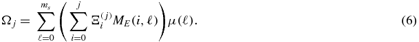
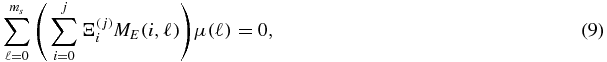
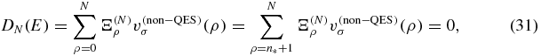
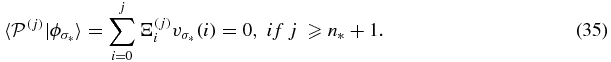
Implementation of OPPQ requires that the Hamiltonian in question admit a moment equation representation either in the x-coordinate or in some transformed coordinate space. In this work, the power moments for the Ψ-representation are defined by μ(p) ≡ ∫dx x^pΨ(x). The Schrödinger equation will be converted into a recursive moment equation. It corresponds to an m_s + 1 order finite difference equation in which the first m_s + 1 moments (i.e. the missing moments [14]) generate all the other moments through a linear relation involving known, energy dependent, coefficients:

$$\begin{equation} \mu (p) = \sum _{\ell = 0}^{m_s} M_E(p,\ell ) \ \mu (\ell ), \end{equation} \tag{ 1 }$$

p ⩾ 0. The following presents a more streamlined development of OPPQ than that originally communicated in [11, 12]. In addition, it will serve to define the necessary components of our analysis.

The orthogonal polynomial projection quantization formalism. Suppose $\mathcal{R}(x) > 0$ is a positive, bounded, configuration admitting an infinite set of orthonormal polynomials

$$\begin{eqnarray} &&\langle \mathcal{P}^{(j_1)}| \mathcal{R}|\mathcal{P}^{(j_2)}\rangle \equiv \int {\rm d}x \mathcal{P}^{(j_1)}(x) \mathcal{P}^{(j_2)}(x) \mathcal{R}(x) = \delta _{j_1,j_2}, \nonumber \\ &&\mathcal{P}^{(j)}(x) = \sum _{i = 0}^j \Xi _i^{(j)} x^i, \qquad {\rm where} \quad \Xi _j^{(j)} \ne 0. \end{eqnarray} \tag{ 2 }$$

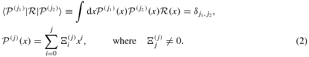
The orthonormal polynomials can be generated, in their monic form, through the standard three-term recursion relation, given the power moments of the reference function, $\mathcal{R}$.

Assume that the non-orthogonal basis $\lbrace \mathcal{P}^{(j)}(x) \mathcal{R}(x)|j\ge 0 \rbrace$ is sufficiently complete that the physical states of interest can be expanded as

$$\begin{eqnarray} &&\Psi (x) = \sum _{j=0}^\infty \Omega _j \mathcal{P}^{(j)}(x) \ \mathcal{R}(x). \end{eqnarray} \tag{ 3 }$$

One can then project out the expansion coefficients exactly:

$$\begin{eqnarray} \Omega _j & = & \int {\rm d}x \ \mathcal{P}^{(j)}(x) \Psi (x) , \end{eqnarray} \tag{ 4 }$$

$$\begin{eqnarray} \Omega _j & = & \sum _{i=0}^j \Xi ^{(j)}_i \mu (i) , \end{eqnarray} \tag{ 5 }$$

$$\begin{eqnarray} \Omega _j & = & \sum _{\ell = 0}^{m_s} \Bigg( \sum _{i = 0}^j\Xi ^{(j)}_i M_E(i,\ell )\Bigg) \mu (\ell ). \end{eqnarray} \tag{ 6 }$$

Now consider the positive (and assumed finite) integral expression $\int {\rm d}x {{\Psi ^2(x)}\over {\mathcal{R}(x)}} < \infty$. We obtain

$$\begin{equation} \int {\rm d}x {{\Psi ^2(x)}\over {\mathcal{R}(x)}}= \sum _{j = 0}^\infty \Omega _j^2 < \infty , \end{equation} \tag{ 7 }$$

resulting in

$$\begin{equation} \lim _{j \rightarrow \infty }\Omega _j = 0. \end{equation} \tag{ 8 }$$

The integral condition in equation (7) can be satisfied if $\mathcal{R}$ decays slower than Ψ²(x) allowing the ratio to be integrable. A less precise condition suggests that if $\mathcal{R}$ decreases as, or slower than, the controlling asymptotic form of Ψ, then equation (8) is satisfied.

The asymptotic behavior of equation (8) suggests that we impose these conditions, at finite order, on appropriate, successive, projection expressions as represented in equation (6):

$$\begin{eqnarray} &&\sum _{\ell = 0}^{m_s} \Bigg ( \sum _{i = 0}^j\Xi ^{(j)}_i M_E(i,\ell )\Bigg ) \mu (\ell ) = 0, \end{eqnarray} \tag{ 9 }$$

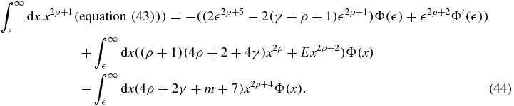
for j = N, N + 1, N + 2, ..., N + m_s, defining an (m_s + 1) × (m_s + 1) determinantal condition:

$$\begin{eqnarray} &&D_N(E) = {\rm Det}( \mathcal{M}_{\eta ,\ell }^{(N)}(E) ) = 0, \end{eqnarray} \tag{ 10 }$$

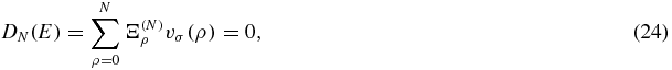
where $\mathcal{M}_{\eta ,\ell }^{(N)}(E) = \sum _{i = 0}^{N+\eta }\Xi ^{(N+\eta )}_i M_E(i,\ell )$. We note that the degree of D_N(E), generally a rational polynomial of the energy , grows as N → ∞, allowing for the generation of converging approximants to all the discrete states.

We also note that OPPQ does not require the reference function to be analytic (as will be the case in our second example). It could be non-differentiable, piece-wise continuous, etc. This allows the reference function to incorporate any non-analytic factors consistent with the form of the physical wavefunction. In particular, any indicial exponent factors can be incorporated within it. An interesting, unpublished, observation concerns the quartic anharmonic oscillator potential as discussed in [11]: V(x) = x⁴ + mx². One can take $\mathcal{R}(x) = {\rm e}^{-{{|x|^3}\over 3}}$. The results are superior to those using the Gaussian as a reference function. In general, OPPQ's convergence improves, the more the reference function imitates the asymptotic form of the solution.

Another important observation is that we do not need the explicit form of $\mathcal{R}(x)$; only the explicit form for the moments are required, since the orthogonal polynomials are generated from them through the well known three-term recursion relation. Thus, one can envision solving for the power moments of the ground state solution and using these to implement OPPQ on the excited states. This is possible through several methods. Of relevance to this work is the eigenvalue moment method (EMM) [14]. It can give tight bounds on the ground state energy, as well as on the power moments [14–16]. It is the first application of semidefinite programming (SDP) to quantum operators [17, 18], although the specific computational implementation in subsequent works [15, 16] exploited linear programming, convex optimization, methods. Advances in SDP algorithms have led to more recent applications in combinatorics [19] and many body physics [20, 21]. Other works on (asymptotic analysis based) moment quantization include those of Killingbeck et al [22] and Blankenbecler et al [23].

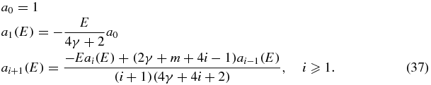
Exactness of OPPQ conditions for QES states. The last equation, equation (10), represents the OPPQ conditions applicable to any state. However, for QES states, these conditions are exact. This follows from the fact that if the QES state is of the form $\Psi _{{\rm QES}}(x) = P_d(x) \mathcal{R}(x)$ then

$$\begin{eqnarray} &&\Psi _{{\rm QES}}(x) = P_d(x) \mathcal{R}(x) = \sum _{j=0}^d c_j \mathcal{P}^{(j)}(x) \mathcal{R}(x), \end{eqnarray} \tag{ 11 }$$

and

$$\begin{eqnarray} &&\langle \mathcal{P}^{(j)}|\Psi _{{\rm QES}}\rangle = 0, \quad {\rm if}\quad j \ge d+1. \end{eqnarray} \tag{ 12 }$$

That is, the OPPQ conditions are exactly satisfied for QES states, provided the OPPQ order N ⩾ d + 1, as given in equations (9) and (10). Thus, using the QES controlling asymptotic factor as the reference function allows us to generate both QES and non-QES states through the same computational procedure. Furthermore, the QES results are exact, to all order N ⩾ d + 1 (will remain unchanged). For the non-QES states, as the OPPQ order, N, increases, the approximate non-QES energies will converge exponentially fast to the true physical values.

Generating explicit closed form QES-energies. One can solve equation (12) algebraically for the QES states. We do not pursue this here. Instead, we give the numerical results for both QES and non-QES states which confirms the above discussion. Instead, if one wants to generate closed form expressions for the energies, we must work within the representation:

$$\begin{eqnarray} \Phi (x) & \equiv & \mathcal{R}(x) \Psi (x), \end{eqnarray} \tag{ 13 }$$

and implement an OPPQ analysis using the moment equation for Φ, which is assumed to exist. We will denote the moments of Φ by ν(p) ≡ ∫dx x^pΦ(x). The OPPQ analysis now involves the orthonormal polynomials of $\mathcal{R}^2(x)$. All proceeds as in the Ψ representation. We refer to each as OPPQ-Ψ and OPPQ-Φ. The one big advantage of OPPQ-Φ is that the explicit form for the energies, and the manifestation of the Bender–Dunne orthogonal polynomials in the energy become transparent. This is because within the representation in equation (13) the underlying moment equation can be reduced to a zero missing moment problem, m_s = 0, greatly simplying the OPPQ algebraic analysis (i.e. a 1 × 1 determinant matrix is involved).

In the following sections we implement OPPQ-Ψ and OPPQ-Φ on both the sextic anharmonic oscillator potential, V_sa(x), and the singular sextic potential, V_ss(x), defined earlier.

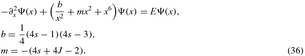
The sextic anharmonic oscillator Schrödinger equation is

$$\begin{equation} {-}\partial _x^2\Psi (x) + (g x^6 + b x^4 + m x^2) \Psi (x) = E \Psi (x). \end{equation} \tag{ 14 }$$

For the physical bound states, multiplying both sides by x^p and integrating over the entire real axis, after performing the necessary integration by parts, yields the moment equation

$$\begin{eqnarray} &&g\mu (p+6) = -b\mu (p+4) -m\mu (p+2) + E\mu (p) +p(p-1)\mu (p-2), \end{eqnarray} \tag{ 15 }$$

for p ⩾ 0. All the moments are linearly dependent on the first six moments {μ(0), ..., μ(5)} corresponding to missing moment order m_s = 5. This leads to a 6 × 6 OPPQ determinant.

Since parity is conserved, there must be even and odd states indexed by σ = 0, 1, respectively. The even and odds states satisfy μ_e(odd) = 0 and μ_o(even) = 0, respectively. We can exploit this and work within an alternate moment equation representation that specifically projects out the odd or even states, respectively.

Let ξ ≡ x², hence $\mu _e(2\rho ) \equiv u_e(\rho ) = \int _0^\infty {\rm d}\xi \ \xi ^{\rho -{1\over 2}} \Psi _e(\sqrt{\xi })$. The resulting moment equation is

$$\begin{eqnarray} &&g u_e(\rho +3) = -b u_e(\rho +2) -m u_e(\rho +1) + E u_e(p) +2\rho (2\rho -1) u_e(\rho -1), \end{eqnarray} \tag{ 16 }$$

for ρ ⩾ 0. The missing moment order is now m_s = 2 resulting in a 3 × 3 OPPQ determinant.

For the odd states, one has $\mu _o(2\rho +1) \equiv u_o(\rho ) = \int _0^\infty {\rm d}\xi \ \xi ^{\rho } \Psi _o(\sqrt{\xi })$ with moment equation

$$\begin{eqnarray} &&g u_o(\rho +3) = -b u_o(\rho +2) -m u_o(\rho +1) + E u_o(p) +2\rho (2\rho +1) u_e(\rho -1), \end{eqnarray} \tag{ 17 }$$

for ρ ⩾ 0. Again m_s = 2 with an OPPQ determinant that is 3 × 3.

The QES states are represented by $\Psi (x) = P_d(x)\mathcal{R}_{{\rm sa}}(x)$, where $\mathcal{R}_{sa}(x) = {\rm e}^{-{{\sqrt{g}}\over 4} (x^4 +{b\over g} x^2)}$, as determined by a JWKB analysis. We note that our notation only emphasizes the degree of the polynomial. It will turn out that different QES states can have the same polynomial degree 'd' (with varying polynomial form and varying numbers of real roots). Our notation implicitly allows for this variation.

Let d = 2n + σ = integer ⩾ 0. A given set of potential parameter values {g, b, m} will admit QES states if the following condition is satisfied:

$$\begin{equation} g^{3\over 2} (8(2n + \sigma )+12) +4mg-b^2 = 0. \end{equation} \tag{ 18 }$$

It is to be emphasized that equation (18) only determines the degree of the polynomial for the QES state: d = 2n + σ.

We note that any integer pair (n, σ) that satisfy equation (18) is unique, since if it were not then the differences would have to satisfy 2Δn + Δσ = 0. Since Δσ = 0, ±1, one cannot find another integer pair.

It also happens that equation (18) defines a condition for a special subset of non-QES states. This will become readily apparent within the OPPQ-Ψ formulation in the next section. That is, they too will be characterized by the same integer pair (n, σ); however the 'n' index does not correspond to there being a polynomial factor for the corresponding wavefunction. Instead, the Fourier transform will be associated with a k^{d + 2} factor (refer to the theorem in the next section). We will use the asterisk (n_*, σ_*) to implicitly refer to the integer pair satisfying equation (18) that correspond to the QES states.

In the next section (and in the appendix) we argue that if equation (18) is satisfied by a particular pair {n_*, σ_*}, then there must be 'n_* + 1' QES states, all having the same polynomial degree, d_* = 2n_* + σ_*. Furthermore the QES states are the n_* + 1 lowest energy states for the corresponding parity σ_*.

The easiest way to determine equation (18) and the number of QES states is to examine under what conditions the ratio ${\Psi \over {\mathcal{R}_{{\rm sa}}}}$ truncates (i.e. the Taylor–Hill expansion). Another direct approach is through OPPQ-Φ to be presented in the following section. In principle, the same can be realized through equation (10), although the underlying algebraic analysis may be more complicated (since m_s > 0). In this section, we simply test the effectiveness of OPPQ-Ψ in generating both the non-QES states, as well as the QES states. We emphasize that the sextic anharmonic oscillator in question will admit non-QES states when equation (18) is not satisfied; and will also admit non-QES states (of the same σ_* symmetry), when equation (18) is satisfied. The more interesting case is the second.

For completeness, we also note that equation (18) can be inferred from JWKB analysis and tested through OPPQ-Ψ. Thus, from first order JWKB we have $\Psi (x) \sim {1\over {({\partial _xS(x))^{1\over 2}}}} \exp(-S(x))$, where

$$\begin{equation} S(x) = {\sqrt{g}\over 4}\left(x^4 +{b\over g} x^2\right) + {1\over {\sqrt{g}}} \left({m\over 2} -{{b^2}\over {8g}} \right)\,{\rm Ln}(x). \end{equation} \tag{ 19 }$$

The leading asymptotic form becomes $\Psi _{\sigma }(x) \sim x^{d} \mathcal{R}_{{\rm sa}}(x)$, where the non-exponential factor is determined by the parameter $d = {1\over {\sqrt{g}}} \big( {{b^2}\over {8g}}-{m\over 2}\big)-{3\over 2}$. Since this parameter identifies the dominant power, which must be an integer for QES states, and there must be even and odd solutions, the potential function parameters leading to an integer form for d = 2n_* + σ_* correspond to the QES potential function constraints in equation (18).

Within the $u_e(\rho ) \equiv \int _0^\infty {\rm d}\xi \ \xi ^\rho \phi _e(\xi )$ moment representations, the QES even parity states on the positive ξ axis become $\phi _e(\xi ) \equiv {1\over {\sqrt{\xi }}}\Psi _e(\sqrt{\xi }) = P_{d}(\sqrt{\xi }){1\over {\sqrt{\xi }}}\mathcal{R}_{{\rm sa}}(\sqrt{\xi })$. The effective reference function is ${1\over {\sqrt{\xi }}}\mathcal{R}_{{\rm sa}}(\sqrt{\xi })$, where $\mathcal{R}_{{\rm sa}}(\sqrt{\xi }) = {\rm e}^{-{{\sqrt{g}}\over 4} (\xi ^2 +{b\over g} \xi)}$. The polynomial becomes $P_{d}(\sqrt{\xi }) = {\tilde{P}}_{d_e}(\xi )$, a polynomial of degree d_e = n_*. The OPPQ relations in equation (10) now apply with respects to the d_e index. That is, even parity QES states correspond to N_e ⩾ d_e + 1.

Within the $u_o(\rho )\equiv \int _0^\infty {\rm d}\xi \ \xi ^\rho \phi _o(\xi )$ moment representation, the odd QES states correspond to $\phi _o(\xi ) \equiv \Psi _o(\sqrt{\xi }) = P_{d}(\sqrt{\xi }) \mathcal{R}_{{\rm sa}}(\sqrt{\xi }) = {\tilde{P}}_{d_o}(\xi )\sqrt{\xi }\mathcal{R}_{{\rm sa}}(\sqrt{\xi })$, with effective reference function $\sqrt{\xi }\mathcal{R}_{{\rm sa}}(\sqrt{\xi })$, and d_o = n_*. The OPPQ conditions in equation (10) now correspond to N_o ⩾ d_o + 1, where d_o = n_*.

Numerical examples. Consider the potential function parameters g = 1, b² = 8, then for arbitrary {n_*, σ_*} integer values, QES states exist for m = −(4n_* + 2σ_* + 1). Tables 1 and 2 give the OPPQ analysis for the corresponding QES and non-QES states for n_* = 3, as developed within the 3 × 3 OPPQ determinant formalism based on the u_e and u_o moments. It will be noted that as soon as N_{e, o} ⩾ n_* + 1 = 4, the QES states are exactly determined and remain the same constant roots for the corresponding $D_{N_{e,o}}(E)$ function. The other OPPQ energy roots for $D_{N_{e,o}}(E)$ converge to the non-QES states. We emphasize that the numbers given for the QES states represent the first six-seven decimal places of the exact energies with no rounding off. We also give the OPPQ estimate for the non-QES states, derived from a higher order OPPQ analysis using orthonormal polynomials of exp ( − x⁴/4) as developed in [11]. These are associated with N = ∞ entries.

Table 1. Convergence of OPPQ-Ψ (QES* and non-QES) for the first six (even) energy levels of equation (16), g = 1, $b=\sqrt{8}$, m = −(4n_* + 2σ_* + 1), n_* = 3, σ_* = 0.

Ne	$E_0^*$	$E_2^*$	$E_4^*$	$E_6^*$	E8	E10
V(x) = gx6 + bx4 + mx2, $\mathcal{R}_{{\rm sa}}(x) = \exp\big ( {-}{{\sqrt{g}}\over 4}\big (x^4 +{b\over g} x^2\big )\Big )$
1	−3.500 501
2	−6.604 075	0.507 807
3	−4.538 891	2.361 563	8.006 481
4	−4.701 631	2.289 850	13.186 912	28.822 848
5	−4.701 631	2.289 850	13.186 912	28.822 848	61.179 448
6	−4.701 631	2.289 850	13.186 912	28.822 848	51.599 563	102.816 240
7	−4.701 631	2.289 850	13.186 912	28.822 848	48.712 815	82.421 165
8	−4.701 631	2.289 850	13.186 912	28.822 848	47.857 837	74.249 292
9	−4.701 631	2.289 850	13.186 912	28.822 848	47.652 156	70.817 047
10	−4.701 631	2.289 850	13.186 912	28.822 848	47.616 909	69.545 484
11	−4.701 631	2.289 850	13.186 912	28.822 848	47.614 022	69.227 821
12	−4.701 631	2.289 850	13.186 912	28.822 848	47.613 850	69.232 777
∞					47.613 209	69.043 247

Table 2. Convergence of OPPQ-Ψ (QES* and non-QES) for the first six (odd) energy levels of equation (17), g = 1,$b=\sqrt{8}$, m = −(4n_* + 2σ_* + 1),n_* = 3, σ_* = 1.

No	$E_1^*$	$E_3^*$	$E_5^*$	$E_7^*$	E9	E11
V(x) = gx6 + bx4 + mx2, $\mathcal{R}_{{\rm sa}}(x) = \exp\big ( -{{\sqrt{g}}\over 4}\big (x^4 +{b\over g} x^2\big )\Big )$
1	−8.086 559
2	−7.931 590	−0.067 843
3	−6.466 044	5.685 330	10.297 850
4	−6.629 227	4.618 850	18.024 593	34.897 472
5	−6.629 227	4.618 850	18.024 593	34.897 472	70.431 224
6	−6.629 227	4.618 850	18.024 593	34.897 472	59.527 051	114.774 703
7	−6.629 227	4.618 850	18.024 593	34.897 472	56.100 032	92.408 733
8	−6.629 227	4.618 850	18.024 593	34.897 472	55.025 448	83.209 865
9	−6.629 227	4.618 850	18.024 593	34.897 472	54.745 576	79.194 992
10	−6.629 227	4.618 850	18.024 593	34.897 472	54.689 889	77.548 343
∞					54.686 459	76.977 398

For completeness, tables 3 and 4 give both QES and non-QES states derived without working in the explicit parity subspaces. That is, we work with the μ moments directly (m_s = 5), generating the corresponding (6 × 6) OPPQ determinantal equation. The N parameter quoted is different from that in tables 1 and 2. For tables 3 and 4, for the n_* = 3 case, the QES states have P_d(x) with d = 2n_* + σ_*; hence the exact QES energies become manifest for N ⩾ 7 or 8, depending on the even or odd states, respectively.

Table 3. Unified OPPQ-Ψ analysis within μ representation for σ_* = 0, n_* = 3, $b=\sqrt{8}$ and m = −13. QES states $E_0^*$, $E_2^*$, $E_4^*$ and $E_6^*$ are 'exact', while the other states converge fast.

N	$E_0^*$	E1	$E_2^*$	E3	$E_4^*$	E5	$E_6^*$	E7
1	−3.500 501 906 77
2	−6.031 693 117 24	−3.500 501 906 77
3	−6.604 075 482 95	−6.031 693 117 24	0.507 807 963 155
4	−6.604 075 482 95	−4.721 132 090 85	0.507 807 963 155	2.257 090 853 40
5	−4.721 132 090 85	−4.538 891 821 50	2.257 090 853 40	2.361 563 118 23	8.006 481 296 16
6	−4.538 891 821 50	−4.218 873 922 29	2.361 563 118 23	7.103 732 218 95	8.006 481 296 16	16.722 951 8999
7	−4.701 631 222 88	−4.218 873 922 29	2.289 850 024 68	7.103 732 218 95	13.186 912 5971	16.722 951 8999	28.822 848 3475
8	−4.701 631 222 88	−4.257 209 122 89	2.289 850 024 68	6.714 399 422 30	13.186 912 5971	20.249 728 3402	28.822 848 3475	43.747 556 3324
9	−4.701 631 222 88	−4.257 209 122 89	2.289 850 024 68	6.714 399 422 30	13.186 912 5971	20.249 728 3402	28.822 848 3475	43.747 556 3324
10	−4.701 631 222 88	−4.258 005 706 49	2.289 850 024 68	6.714 310 045 95	13.186 912 5971	20.535 288 3528	28.822 848 3475	39.213 766 8519
11	−4.701 631 222 88	−4.258 005 706 49	2.289 850 024 68	6.714 310 045 95	13.186 912 5971	20.535 288 3528	28.822 848 3475	39.213 766 8519
12	−4.701 631 222 88	−4.258 010 759 80	2.289 850 024 68	6.715 033 706 68	13.186 912 5971	20.560 899 7790	28.822 848 3475	38.149 722 1283
13	−4.701 631 222 88	−4.258 010 759 80	2.289 850 024 68	6.715 033 706 68	13.186 912 5971	20.560 899 7790	28.822 848 3475	38.149 722 1283
14	−4.701 631 222 88	−4.258 007 810 19	2.289 850 024 68	6.715 123 974 19	13.186 912 5971	20.562 204 4115	28.822 848 3475	37.909 138 9572
15	−4.701 631 222 88	−4.258 007 810 19	2.289 850 024 68	6.715 123 974 19	13.186 912 5971	20.562 204 4115	28.822 848 3475	37.909 138 9572
16	−4.701 631 222 88	−4.258 007 437 07	2.289 850 024 68	6.715 129 898 94	13.186 912 5971	20.562 079 5974	28.822 848 3475	37.867 255 6901
17	−4.701 631 222 88	−4.258 007 437 07	2.289 850 024 68	6.715 129 898 94	13.186 912 5971	20.562 079 5974	28.822 848 3475	37.867 255 6901
18	−4.701 631 222 88	−4.258 007 416 21	2.289 850 024 68	6.715 129 759 00	13.186 912 5971	20.562 035 4769	28.822 848 3475	37.862 623 9770
19	−4.701 631 222 88	−4.258 007 416 21	2.289 850 024 68	6.715 129 759 00	13.186 912 5971	20.562 035 4769	28.822 848 3475	37.862 623 9770

Table 4. Unified OPPQ-Ψ analysis within μ representation for σ_* = 1, n_* = 3,$b=\sqrt{8}$ and m = −15. QES states $E_1^*$, $E_3^*$, $E_5^*$ and $E_7^*$ are 'exact', while the other states converge fast.

N	E0	$E_1^*$	E2	$E_3^*$	E4	$E_5^*$	E6	$E_7^*$	E8
1	−4.319 621 151 62
2	−8.086 559 878 11	−4.319 621 151 62
3	−9.550 873 560 79	−8.086 559 878 11	−0.190 781 182 520
4	−9.550 873 560 79	−7.931 590 138 29	−0.190 781 182 520	−0.067 843 386 2236
5	−7.931 590 138 29	−6.517 604 110 99	−0.067 843 386 2236	0.055 477 759 4537	4.599 253 523 08
6	−6.517 604 110 99	−6.466 044 956 81	0.055 477 759 4537	4.599 253 523 08	5.685 330 084 05	10.297 850 4560
7	−6.840 978 184 74	−6.466 044 956 81	1.077 497 984 10	5.685 330 084 05	10.297 850 4560	11.726 737 4340	20.922 125 8143
8	−6.840 978 184 74	−6.629 227 918 05	1.077 497 984 10	4.618 850 269 29	11.726 737 4340	18.024 593 2316	20.922 125 8143	34.897 472 6626
9	−6.849 012 989 88	−6.629 227 918 05	1.018 681 431 68	4.618 850 269 29	10.934 182 0352	18.024 593 2316	25.617 223 7107	34.897 472 6626	51.487 444 8871
10	−6.849 012 989 88	−6.629 227 918 05	1.018 681 431 68	4.618 850 269 29	10.934 182 0352	18.024 593 2316	25.617 223 7107	34.897 472 6626	51.487 444 8871
11	−6.849 395 797 45	−6.629 227 918 05	1.017 240 283 94	4.618 850 269 29	10.928 335 0058	18.024 593 2316	26.018 696 4925	34.897 472 6626	46.161 784 6405
12	−6.849 395 797 45	−6.629 227 918 05	1.017 240 283 94	4.618 850 269 29	10.928 335 0058	18.024 593 2316	26.018 696 4925	34.897 472 6626	46.161 784 6405
13	−6.849 411 336 96	−6.629 227 918 05	1.017 215 758 01	4.618 850 269 29	10.929 156 5335	18.024 593 2316	26.059 739 4744	34.897 472 6626	44.846 729 0999
14	−6.849 411 336 96	−6.629 227 918 05	1.017 215 758 01	4.618 850 269 29	10.929 156 5335	18.024 593 2316	26.059 739 4744	34.897 472 6626	44.846 729 0999
15	−6.849 411 286 33	−6.629 227 918 05	1.017 219 963 10	4.618 850 269 29	10.929 299 4586	18.024 593 2316	26.062 582 7763	34.897 472 6626	44.527 287 8301
16	−6.849 411 286 33	−6.629 227 918 05	1.017 219 963 10	4.618 850 269 29	10.929 299 4586	18.024 593 2316	26.062 582 7763	34.897 472 6626	44.527 287 8301
17	−6.849 411 184 33	−6.629 227 918 05	1.017 220 655 44	4.618 850 269 29	10.929 312 1992	18.024 593 2316	26.062 511 7133	34.897 472 6626	44.465 879 9515
18	−6.849 411 184 33	−6.629 227 918 05	1.017 220 655 44	4.618 850 269 29	10.929 312 1992	18.024 593 2316	26.062 511 7133	34.897 472 6626	44.465 879 9515
19	−6.849 411 172 46	−6.629 227 918 05	1.017 220 707 55	4.618 850 269 29	10.929 312 4794	18.024 593 2316	26.062 450 1552	34.897 472 6626	44.457 916 3980

If one works within the representation $\Phi (x) = \mathcal{R}_{{\rm sa}}(x) \Psi (x)$, the sextic anharmonic oscillator problem becomes an m_s = 0 moment equation, facilitating the generation of closed form expressions for the QES energies, etc. The controlling asymptotic form is $\mathcal{R}_{{\rm sa}}^2(x)$. The corresponding differential equation becomes

$$\begin{eqnarray} &&{-}\partial _x^2\Phi - \bigg({b\over {\sqrt{g}}} x + 2 \sqrt{g} x^3\bigg) \partial _x \Phi (x) + \bigg(\bigg(m-3\sqrt{g} -{{b^2}\over {4g}}\bigg)x^2 - \bigg(E+ {b\over {2\sqrt{g}} } \bigg)\bigg) \Phi (x) = 0.\nonumber\\ \end{eqnarray} \tag{ 20 }$$

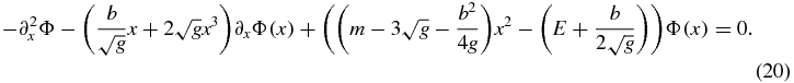
The power moments for the physical states ν(p) = ∫dx x^pΦ(x) satisfy the moment equation:

$$\begin{eqnarray} &&\bigg(m+3\sqrt{g} -{{b^2}\over {4g}} +2 \sqrt{g} p)\bigg) \nu (p+2) \nonumber \\ &&=\bigg(E- {b\over {\sqrt{g}}} \bigg(p+{1\over 2}\bigg)\bigg)\nu (p) + p(p-1)\nu (p-2), \quad p \ge 0. \end{eqnarray} \tag{ 21 }$$

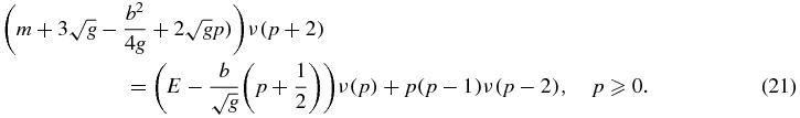
This defines an m_s = 1 missing moment problem; however given that the physical system admits parity invariant states, the moment equation decouples into the corresponding even and odd order power moments.

Define v_{e, o}(ρ) = ν(2ρ + σ), σ = 0, 1, for the even and odd cases, respectively. This means that upon transforming into the independent variable ξ ≡ x², the even states $\Phi _e(x) \rightarrow \phi _e(\xi ) \equiv {1\over \sqrt{\xi }}\Phi _e(\sqrt{\xi })$, and $\Phi _o(x) \rightarrow \phi _o(\xi ) \equiv \Phi _o(\sqrt{\xi })$. For the QES states these take on the form $\phi _{e,o}(\xi ) = {\tilde{P}}_{n_*}(\xi ) \xi ^{ {{2\sigma -1}\over 2} }\mathcal{R}^2_{{\rm sa}}(\sqrt{\xi })$, where the non-polynomial factors define the effective reference function. The corresponding moment equations become (i.e. $v_\sigma (\rho ) = \int _0^\infty {\rm d}\xi \ \xi ^\rho \phi _\sigma (\xi )$):

$$\begin{eqnarray} &&\bigg(m -{{b^2}\over {4g}} + \sqrt{g}(4 \rho + 3 + 2\sigma )\bigg) v_{\sigma }(\rho +1) \nonumber \\ &&=\bigg(E- {b\over {\sqrt{g}}}\bigg(2\rho +{1\over 2}+\sigma \bigg)\bigg)v_{\sigma }(\rho ) + 2\rho (2\rho -1+2 \sigma ) v_{\sigma }(\rho -1), \end{eqnarray} \tag{ 22 }$$

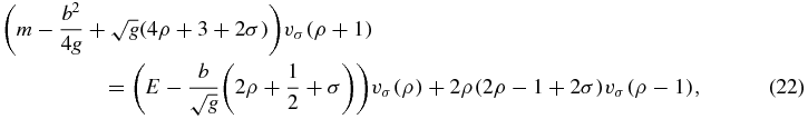
ρ ⩾ 0, and σ = 0, 1. These correspond to m_s = 0 and the OPPQ determinant is 1 × 1 energy dependent function. Define the coefficient on the left-hand side as

$$\begin{eqnarray} C_{\sigma ;1}(m,b,g;\rho +1) & = & m - {{b^2}\over {4g}} + \sqrt{g}(4\rho +3+2\sigma ). \end{eqnarray} \tag{ 23 }$$

Except for anomalous (but important) values of the potential function parameters the (m_s = 0) recursive nature of the moment equations leads to the conclusion that if v_σ(0) ≠ 0 (i.e. we take v_σ(0) ≡ 1), then v_σ(ρ) is a polynomial of degree ρ in the energy variable E. Under these conditions, the OPPQ-Φ determinant condition is defined by the energy dependent function (i.e. since m_s = 0 then M_E(ρ, 0) = v_σ(ρ))

$$\begin{eqnarray} &&D_N(E) = \sum _{\rho = 0}^N\Xi ^{(N)}_\rho v_\sigma (\rho ) = 0, \end{eqnarray} \tag{ 24 }$$

where the $\Xi ^{(N)}_\rho$ are the orthonormal polynomial coefficients for the effective reference functions $\xi ^{ {{2\sigma -1}\over 2} } \mathcal{R}^2_{{\rm sa}}(\sqrt{\xi })$.

The condition that v_σ(0) ≠ 0 is certainly true for the lowest energy state within each parity subspace, since the underlying Sturm–Liouville character of the problem guarantees that the corresponding wavefunction must be a nonnegative function with all its power moments being positive [14].

For a given set of potential function parameters, if C_{σ; 1}(m, b, g; ρ + 1) ≠ 0 for all ρ ⩾ 0, allowing the generation of all moments, then all bound states must satisfy v_σ(0) ≠ 0. If not, then all the power moments for that bound state are zero, suggesting that the state does not exist. This is because the physical states have an analytic Fourier transform whose expansion depends on the power moments. Therefore, the more interesting cases are those where the potential function parameters result in equation (23) becoming zero for some ρ = n.

Now define the (non-monic) polynomials,

$$\begin{eqnarray} &&P_{\sigma }^{(\rho )}(E) \equiv C_{\sigma ;1}(m,b,g;\rho ) \ v_{\sigma }(\rho ). \end{eqnarray} \tag{ 25 }$$

which satisfy a three-term recursion relation (so long as the potential parameters do not produce zero denominators):

$$\begin{eqnarray} &&P_{\sigma }^{(\rho +1)}(E) = { { \big(E-{b\over {\sqrt{g}}}\big(2\rho +{1\over 2}+\sigma \big)\big)} \over {C_{\sigma ;1}(m,b,g;\rho )} } P_{\sigma }^{(\rho )}(E) + {{2\rho (2\rho -1+2\sigma )}\over {C_{\sigma ;1}(m,b,g;\rho -1)}} P_{\sigma }^{(\rho -1)}(E) , \end{eqnarray} \tag{ 26 }$$

for 0 ⩽ ρ < ∞.

Unlike the OPPQ-Ψ formulation, the moment equation in equation (22) displays an anomalous behavior depending on the potential function parameters. Assume that the potential function parameters satisfy C_{σ; 1}(m, b, g; ρ + 1) = 0, for some integer ρ = n_* and parity state σ_*. Since the lowest energy state for the system, within the σ_*-parity subspace, corresponds to a nonnegative function, then all its moments must be positive. In particular $v_{\sigma _*}(0) > 0$. This means that the corresponding lowest energy state must satisfy the polynomial root condition

$$\begin{eqnarray} &&P_{\sigma _*}^{(n_*+1)}(E) = 0. \end{eqnarray} \tag{ 27 }$$

Since the energy polynomials are known in closed form, the lowest state energy is also known in closed form in the sense of being a root of this known polynomial. This analysis was originally discovered in the context of the EMM, which solely focused on the lowest energy states within each parity subspace [14]. Since the thrust of EMM was to use convex optimization methods to bound the eigenenergies associated with nonnegative wavefunction configurations, the significance of the other n_* energy roots to equation (27), within each parity subspace, was not communicated. We do so here. In the appendix we give a simple proof (originally developed within the EMM analysis) why the conditions

$$\begin{eqnarray} &&C_{\sigma _*;1}(m,b,g;n_*+1) = m - {{b^2}\over {4g}} + \sqrt{g}(4n_*+3+2\sigma _*) = 0, \end{eqnarray} \tag{ 28 }$$

generates all the first n_* + 1 QES states (those whose energies can be determined in closed form as the roots of known polynomials). Clearly this is the same condition in equation (18). We reemphasize the fact that if equation (28) is satisfied, or equivalently equation (27), then the n_* + 1 lowest energy states are QES states. Furthermore, the proof also argues why the zeroth moment of the QES states cannot be zero:

$$\begin{eqnarray} &&v_{\sigma _*}(0) \ne 0, {\rm for \ the \ QES \ states.} \end{eqnarray} \tag{ 29 }$$

As noted, if equation (28) is satisfied, then the first n_* + 1 lowest energy states will be QES states (appendix). Since the potential is unbounded from above with infinitely many discrete states of parity σ_*, these non-QES states of the same σ_* parity cannot satisfy equation (29). The only conclusion is that

Theorem. The non-QES states of the same parity as the QES-states (σ = σ_*), must have v_σ(ρ) = 0, for 0 ⩽ ρ ⩽ n_*. That is, $\int {\rm d}x \ x^{2\rho +\sigma _*}\Phi _{\sigma _*}^{({\rm non-QES})}(x) = 0$, for 0 ⩽ ρ ⩽ n_*. This means that within the Φ representation, the wavefunction must behave as: $\Phi _{\sigma }^{({\rm non-QES})}(x) = \partial _x^{2n_*+2+\sigma _*}\Upsilon (x)$, for some even function ϒ. That is, the corresponding, analytic, Fourier transform must be $O(k^{2n_*+2+ \sigma _*})$ at the origin.

A quicker confirmation of this is that when the zero condition in equation (28) is satisfied then the ρ = n_* iterate in the moment equation (equation (22)) becomes

$$\begin{eqnarray} &&\left(\left(E- {b\over {\sqrt{g}}}\left(2\rho +{1\over 2}+\sigma \right)\right)\Lambda _{\sigma _n}(E,n_*) + 2n_*(2n_*-1+2 \sigma _*)\Lambda _{\sigma _*}(E,n_*-1)\right) v_{\sigma }(0) = 0, \nonumber \\ \end{eqnarray} \tag{ 30 }$$

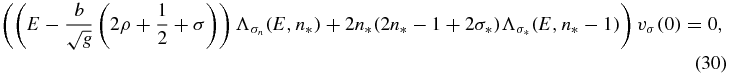
where we have made explicit that v_σ(ρ) = Λ_σ(E, ρ)v_σ(0), involving a polynomial in the energy, so long as ρ ⩽ n_*. Therefore, there are only three possibilities, either the energy must satisfy the underlying polynomial equation (equation (27)) corresponding to the QES states, or v_σ(0) = 0, or both (although not possible according to the proof in the appendix). Therefore, the theorem is confirmed.

Computational implementation of OPPQ-Φ. The sextic anharmonic potential under consideration presents four different potential function parameter regimes.

• Case I: The parameters {g, m, b} do not admit any QES state.
• Case II: If {n_*, σ_*} exist, then all the states of the opposite parity σ ≠ σ_* are non-QES states.
• Case III: If {n_*, σ_*} exist, then within the σ_* parity subspace, there will be infinitely many non-QES states.
• Case IV: If {n_*, σ_*} exist, then within the σ_* parity subspace, there will be n_* + 1 QES states.

Cases I and II represent standard OPPQ-Φ implementation; and quantization is achieved through equation (24). As N → ∞ the roots converge to the true physical values.

Case III is more delicate since the previous theorem requires that the first n_* + 1 moments of the non-QES states of the same parity as the QES states ( σ = σ_*) be zero, or $v_{\sigma }^{({\rm non-QES})}(\rho ) = 0, \rho \le n_*$. Thus the moment equation in equation (22) begins its recursive structure at ρ = n_* + 1. That is, the nonzero moment $v_{\sigma }^{{\rm non\hbox{-}QES}}(n_*+1)$ generates $v_{\sigma }^{{\rm non\hbox{-}QES}}(n_*+2)$, etc. It becomes an effective m_s = 0 missing moment problem. Letting 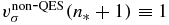$v_{\sigma }^{{\rm non\hbox{-}QES}}(n_*+1) \equiv 1$, the OPPQ-Φ quantization is identical to that for cases I–II:

$$\begin{eqnarray} &&D_N(E) = \sum _{\rho = 0}^N\Xi ^{(N)}_\rho v_{\sigma }^{({\rm non-QES})}(\rho ) = \sum _{\rho = n_*+1}^N\Xi ^{(N)}_\rho v_{\sigma }^{({\rm non-QES})}(\rho ) = 0, \end{eqnarray} \tag{ 31 }$$

where the non-QES states have the same parity as the QES states, σ = σ_*.

Case IV: The QES energies correspond to the zeroes of equation (27).

Alternative option for cases III and IV:. We can bypass the direct use of equation (27) and identify a uniform OPPQ procedure on all states of symmetry σ_*. In the following analysis σ = σ_*; the notation does not discriminate between the QES and non-QES states. We impose OPPQ-Φ on the moment equation in equation (22), omitting the ρ = n_* entry. Thus, the moments {v_σ(ρ)|ρ ⩾ n_* + 2} can be linearly related to {v_σ(n_* + 1), v_σ(n_*)}. However, v_σ(n_*) is linearly related to v_σ(0). Accordingly, we can define the representation

$$\begin{eqnarray} &&v_{\sigma }(\rho ) = M_E(\rho ,n_*+1)v_{\sigma }(n_*+1) + M_E(\rho ,0)v_{\sigma }(0), \end{eqnarray} \tag{ 32 }$$

for ρ ⩾ 0. This is effectively an m_s = 1 problem (i.e. two linear variables). We can now impose the OPPQ-Φ constraints

$$\begin{eqnarray} &&D_N(E) = {\rm Det}\left( \begin{array}{@{}c@{}} \displaystyle\sum _{i=0}^{N} \Xi _i^{(N)}M_E(i,n_*+1) , \displaystyle\sum _{i=0}^{N }\Xi _i^{(N)}M_E(i,0) \\ \displaystyle\sum _{i=0}^{N+1} \Xi _i^{(N+1)}M_E(i,n_*+1) , \displaystyle\sum _{i=0}^{N+1 }\Xi _i^{(N+1)}M_E(i,0)\\ \end{array}\right) = 0. \end{eqnarray} \tag{ 33 }$$

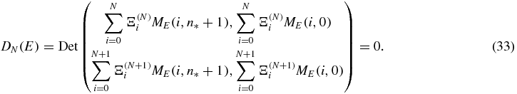
This determinantal equation generates the QES states exactly provided N ⩾ n_* + 1. This is because the QES states must satisfy $\langle \mathcal{P}^{(N)}|\phi _{{\rm QES}}\rangle = 0$, for every N ⩾ n_* + 1 (i.e. we are working within each parity subspace and $\mathcal{P}^{(N)}$ denotes the orthonormal polynomial generating the corresponding Ξ's). The non-QES of the same QES parity, σ_*, must satisfy equation (33), which is an approximation that leads to converging results in the N → ∞ limit. The corresponding solutions, as N → ∞, will display the behavior v_σ(0) → 0, consistent with true form of the non-QES states of σ_* parity. Therefore, D_N(E) factorizes into two polynomials:

$$\begin{eqnarray} &&D_N(E) = P_{({\rm non-QES});\sigma _*}^{(N)}(E) \times P_{\sigma _*}^{(n_*+1)}(E) = 0, \ N \ge n_*+1, \end{eqnarray} \tag{ 34 }$$

where the first polynomial approximates the non-QES state energies (through its real roots), and the second polynomial factor corresponds to the QES polynomial in equation (27), generating all n_* + 1 QES energies, provided N ⩾ n_* + 1.

For completeness, we note that if the QES energy is determined through equation (27), then equation (22) cannot be used to directly generate all the moments, since it truncates at ρ = n_*. That is, the $v_{\sigma _*}(\rho \ge n_*+1)$ moments cannot be determined through equation (22) for the QES states, since $v_{\sigma _*}(n_*+1)$ decouples from the moment equation. However, we can still connect $v_{\sigma _*}(n_*+1)$ to all the lower order moments (and use this in turn to generate all the higher order moments through equation (22)). Since the QES configuration is given by $\phi _{\sigma _*}(\xi ) = {\tilde{P}}_{n_*}(\xi ) \xi ^{ {{2\sigma _*-1}\over 2} }\mathcal{R}^2_{{\rm sa}}(\sqrt{\xi })$ (i.e. the polynomial is implicitly dependent on σ_* as well) the orthonormal polynomials, $\mathcal{P}^{(j)} = \sum _{i=0}^j\Xi _i^{(j)}\xi ^i$, of the effective reference function $\xi ^{ { {2\sigma _*-1}\over 2} }\mathcal{R}^2_{{\rm sa}}(\sqrt{\xi })$ must satisfy the orthogonality properties

$$\begin{eqnarray} &&\langle \mathcal{P}^{(j)}| \phi _{\sigma _*}\rangle = \sum _{i=0}^j\Xi _i^{(j)} v_{\sigma _*}(i) = 0, \ if \ j \ \ge n_*+1 . \end{eqnarray} \tag{ 35 }$$

Therefore, the $v_{\sigma _*}(n_*+1)$ moment can be connected to the lower order moments, since $\Xi _j^{(j)} \ne 0$. This can also be used to generate all the higher order moments in a similar manner, duplicating what would be obtained from the moment equation.

Numerical results. Tables 5 and 6 give the numerical results of OPPQ-Φ for case III (i.e. equation (31)) corresponding to non-QES states of the same parity as the QES states. Tables 7 and 8 show how the extended moment representation in equations (32) and (33), for both QES and non-QES states of the same σ_* parity, also yields consistent results with that in tables 5 and 6. In tables 7 and 8, we compare the QES energies obtained through equation (33) with those directly generated from the roots of the polynomials in equation (27). They are identical (validating the factorization in equation (34)). We also compare the non-QES energies generated through equation (33) with those generated through (31). We expect the non-QES energies in tables 5 and 6 to be more accurate than those approximated through equation (33) as represented in tables 7 and 8, since the former directly incorporate the zero-moment structure identified in the theorem.

Table 5. OPPQ-Φ determination of non-QES states (of σ = σ_* = 0 symmetry) computed by taking v_σ(ρ) = 0, 0 ⩽ ρ ⩽ n_*, and {v_σ(ρ)|ρ ⩾ n_* + 1} satisfy an effective m_s = 0 moment equation. Refer to equation (31).

N	E8	E10	E12	E14
$V(x) = x^6 + \sqrt{8}x^4-13 x^2$, n* = 3, σ* = 0
5	48.394 656
6	47.671 288	72.503 581
7	47.617 135	69.537 633	101.036 761
8	47.613 461	69.101 670	94.571 123	133.727 067
9	47.613 226	69.049 273	93.118 330	122.972 492
10	47.613 211	69.044 300	92.864 698	119.986 303
11	47.613 211	69.044 199	92.856 805	119.850 391

Table 6. OPPQ-Φ determination of non-QES states (of σ = σ_* = 1 symmetry) computed by taking v_σ(ρ) = 0, 0 ⩽ ρ ⩽ n_*, and {v_σ(ρ)|ρ ⩾ n_* + 1} satisfy an effective m_s = 0 moment equation. Refer to equation (31).

N	E9	E11	E13	E15
$V(x) = x^6 + \sqrt{8}x^4-15 x^2$, n* = 3, σ* = 1
5	55.531 291
6	54.750 410	80.668 061
7	54.690 840	77.512 874	110.194 217
8	54.686 737	77.041 110	103.388 049	143.814 626
9	54.686 468	76.982 602	101.807 743	132.398 420
10	54.686 447	76.974 990	101.398 734	127.471 438

Table 7. Comparison of QES and non-QES states, of σ_* = 0 symmetry, computed through the exact root formula $P^{n_*+1}_{\sigma _*}(E^*) = 0$ in equation (27) and OPPQ-Φ Applied to equations (32) and (33). No rounding off for QES energies.

N	$E_0^*$	$E_2^*$	$E_4^*$	$E_6^*$	E8	E10
	−4.701 631	2.289 850	13.186 912	28.822 848	NA	NA
$V(x) = x^6 + \sqrt{8}x^4-13 x^2$, n* = 3, σ* = 0
4	−4.701 631	2.289 850	13.186 912	28.822 848
5	−4.701 631	2.289 850	13.186 912	28.822 848	49.879 720
6	−4.701 631	2.289 850	13.186 912	28.822 848	47.994 447	76.381 590
7	−4.701 631	2.289 850	13.186 912	28.822 848	47.679 059	70.953 850
8	−4.701 631	2.289 850	13.186 912	28.822 848	47.624 584	69.527 914
9	−4.701 631	2.289 850	13.186 912	28.822 848	47.615 172	69.156 251
10	−4.701 631	2.289 850	13.186 912	28.822 848	47.613 408	69.058 368
11	−4.701 631	2.289 850	13.186 912	28.822 848	47.612 358	68.924 938

Table 8. Comparison of QES and non-QES states, of σ_* = 1 symmetry, computed through the exact root formula $P^{n_*+1}_{\sigma _*}(E^*) = 0$ in equation (27) and OPPQ-Φ applied to equations (32) and (33). No rounding off for QES energies.

N	$E_1^*$	$E_3^*$	$E_5^*$	$E_7^*$	E9	E11
	−6.629 227	4.618 850	18.024 593	34.897 472	NA	NA
$V(x) = x^6 + \sqrt{8}x^4-15 x^2$,n* = 3, σ* = 1
4	−6.629 227	4.618 850	18.024 593	34.897 472
5	−6.629 227	4.618 850	18.024 593	34.897 472	56.946 5755
6	−6.629 227	4.618 850	18.024 593	34.897 472	55.048 5775	84.394 5915
7	−6.629 227	4.618 850	18.024 593	34.897 472	54.745 4855	78.850 5925
8	−6.629 227	4.618 850	18.024 593	34.897 472	54.696 0975	77.435 1185
9	−6.629 227	4.618 850	18.024 593	34.897 472	54.688 1985	77.088 5815
10	−6.629 227	4.618 850	18.024 593	34.897 472	54.687 2425	77.034 9865
11	−6.629 227	4.618 850	18.024 593	34.897 472	54.687 3885	77.035 6645

Consider the singular sextic potential problem with a reparameterization of the potential function:

$$\begin{eqnarray} &&{-}\partial _x^2 \Psi (x)+ \Big ({b\over { x^2}} + m x^2 + x^6\Big ) \Psi (x) = E\Psi (x), \nonumber \\ &&b = {1\over 4} (4s-1)(4s-3) , \nonumber \\ &&m = -(4s+4J-2). \end{eqnarray} \tag{ 36 }$$

The wavefunction must assume the form Ψ(x) = x^γA(x²), near the origin. Since the probability density must be integrable it follows that $\gamma > -{1\over 2}$. The indicial equation gives γ² − γ − b = 0, or $\gamma = {{1\pm (4s-2)}\over 2}$. We take $\gamma = 2s-{1\over 2}$.

The QES states should assume the form: $\Psi (x) = P_d(x^2) \mathcal{R}_{{\rm ss}}(x)$ where $\mathcal{R}_{{\rm ss}}(x) = x^\gamma {\rm e}^{-{{x^4}\over 4}}$. As stated before, the objective of OPPQ is not to circumvent the ease with which an x-configuration space analysis brings to determine the QES states, for these one-dimensional problems. Instead, OPPQ defines a unified formalism for simultatenously generating the QES and non-QES states. To this extent, a Taylor–Hill truncation analysis for ${{\Psi (x)}\over {\mathcal{R}_{{\rm ss}}(x)}} \equiv \mathcal{A}(x^2) = \sum _{i=0}^\infty a_i(E) x^{2i}$ gives

$$\begin{eqnarray} &&a_0 = 1 \nonumber \\ &&a_1(E) = -{{E}\over {4\gamma +2}} a_0 \nonumber \\ &&a_{i+1}(E) = {{-E a_i(E) + (2\gamma +m+ 4i-1)a_{i-1}(E)}\over {(i+1)(4\gamma +4i +2)}} ,\quad i \ge 1. \end{eqnarray} \tag{ 37 }$$

We see that in order for $a_{i\ge n_*+2}(E) = 0$ we require

$$\begin{eqnarray} &&4 n_* + 2\gamma +m+ 3 = 0,\qquad {\rm or} \quad J = n_*+1,\nonumber \\ &&a_{n_*+1}(E) = 0. \end{eqnarray} \tag{ 38 }$$

These define the QES states. Thus $\mathcal{A}(x^2) = Polynomial \ of \ degree \ x^{2n_*}\equiv P_{n_*}(x^2)$. That is d = n_*, or $\gamma +2n_* = -{{(m+3)}\over 2}$.

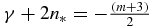The same can be surmized from a JWKB analysis, paralleling that developed in the context of equation (19). Thus $\Psi (x) \sim x^\delta \exp(-{1\over 4} x^4)$, where $\delta = -{{(m+3)}\over 2}$. Comparing with the assumed form $\Psi (x) = P_d(x^2) x^\gamma {\rm e}^{-{{x^4}\over 4}}$ leads to δ = γ + 2d.

We will implement an OPPQ-Ψ analysis before pursuing an OPPQ-Φ formulation. The latter corresponds to $\Phi (x) = \Psi (x) \mathcal{R}_{{\rm ss}}(x) = P_d(x^2) x^{2\gamma }\, {\rm e}^{- {{x^4}\over 2} }$. In both cases, retaining the indicial factor yields moment equations of reduced missing moment order; thereby improving the convergence of the results for the non-QES states. Indeed, keeping the indicial exponent in the Φ representation results in an m_s = 0 problem. All this is best illustrated through several OPPQ-Ψ formulations that attempt to strip the indicial factor, anticipating (erroneously) that there will be improved convergence.

Before implementing OPPQ-Φ, we examine the structure of two OPPQ-Ψ formulations. The first of these involves stripping the wavefunction of the indicial factor: A(x²) = x^−γΨ(x). The second will be to enhance this by multiplying by the physical (exponentially decaying) asymptotic form, ${\tilde{\Phi }}(x^2) = x^{-\gamma }\Psi (x)\, {\rm e}^{-{{x^4}\over 4}}$.

For the first case, we work with the even power moments of A(x²): $u(\rho ) \,{\equiv}\, \int _0^\infty {\rm d}x\, x^{2\rho } A(x^2)$. The relevant differential equation is

$$\begin{eqnarray} &&{-}\partial _x^2A - {{2\gamma }\over x} \partial _x A + (m x^2 +x^6)A = E A. \end{eqnarray} \tag{ 39 }$$

Upon multiplying both sides by x^{2ρ + 2} and integrating by parts we obtain the moment equation

$$\begin{eqnarray} &&u(\rho +4) = - mu(\rho +2) + E u(\rho +1)+ 2(\rho +1-\gamma )(2\rho +1) u(\rho ) , \end{eqnarray} \tag{ 40 }$$

ρ ⩾ 0. We have m_s = 3, resulting in $u(\rho ) = \sum _{\ell = 0}^3M_E(\rho ,\ell ) \ u(\ell )$. The OPPQ analysis is done with respects to the representation $A(x^2) = \sum _{j=0}^\infty \Omega _j \mathcal{P}^{(j)}(x)\, {\rm e}^{-{{x^4}\over 4}}$, involving the orthonormal polynomials of ${\rm e}^{-{{x^4}\over 4}}$. The data in table 9 gives the results for n_* = 3, J = n_* + 1 = 4, s = 1. We emphasize that our objective is not to show the full convergence of the non-QES states, which becomes manifest at higher orders, but to suggest the veracity of our OPPQ analysis as applied to both QES and non-QES states.

Table 9. Comparison of QES and non-QES states computed through the exact root formula a₄(E) = 0 in equation (38) and OPPQ-(x^−γΨ) for m_s = 3 moment equation in equation (40). Parameters s = 1, J = n_* + 1, and n_* = 3.

N	$E_0^*$	$E_1^*$	$E_2^*$	$E_3^*$	E4	E5
	−20.926 277	−6.487 752	+6.487 752	+20.926 277	NA	NA
$V(x) = x^6 + mx^2 + {b\over {x^2}}$, b = 3/2, m = −18
1	−17.752 051
2	−23.465 769	−5.699 531
3	−20.857 859	−8.880 996	4.319 160
4	−20.926 277	−6.487 752	6.487 752	20.926 277
5	−20.926 277	−6.487 752	6.487 752	20.926 277	52.309 013
6	−20.926 277	−6.487 752	6.487 752	20.926 277	41.490 341	94.456 407
7	−20.926 277	−6.487 752	6.487 752	20.926 277	38.426 546	71.311 307
8	−20.926 277	−6.487 752	6.487 752	20.926 277	37.787 371	61.916 009
9	−20.926 277	−6.487 752	6.487 752	20.926 277	37.839 537	58.167 011
36					38.002 392 718	57.536 940 282

The second OPPQ analysis is done on ${\tilde{\Phi }}(x^2) = x^{-\gamma }\Psi (x) \exp(-{{x^4}\over 4})$, which involves the previous representation multiplied by an additional exponential asymptotic form. We obtain the differential equation for ${\tilde{\Phi }}(x^2)$

$$\begin{eqnarray} &&x \partial _x^2{\tilde{\Phi }} +2 ( \gamma +x^4 )\partial _x {\tilde{\Phi }} +(2\gamma -m+3 ) x^3{\tilde{\Phi }} +E x {\tilde{\Phi }} = 0. \end{eqnarray} \tag{ 41 }$$

Upon multiplying both sides by x^{2ρ + 1}, and defining $u(\rho ) = \int {\rm d}x \ x^{2\rho }{\tilde{\Phi }}(x^2)$, we obtain the moment equation:

$$\begin{eqnarray} &&( 4\rho -2\gamma +m+7) u(\rho +2) = E u(\rho +1) + 2(2\rho +1)( \rho +1-\gamma ) u(\rho ), \end{eqnarray} \tag{ 42 }$$

ρ ⩾ 0. So long as γ ≠ integer, we can generate all the power moments and pursue OPPQ for generating the exact QES and (converging) approximate non-QES. The OPPQ representation in this case is ${\tilde{\Phi }}(x) =\sum _{j=0}^\infty \Omega _j \mathcal{O}^{(j)}(x)\, {\rm e}^{-{{x^4}\over 2}}$, where $\mathcal{O}^{(j)}(x)$ are the orthonormal polynomials of ${\rm e}^{-{{x^4}\over 2}}$. The results are given in table 10. The convergence of the non-QES is much faster. The above moment equation almost suggests the manifest existence of QES solutions. However it is not a three-term recursion relation, since the effective missing moment order is m_s = 1.

Table 10. Comparison of QES and non-QES states computed through the exact root formula a₄(E) = 0 in equation (38) and OPPQ-${\tilde{\Phi }}$ for m_s = 1 moment equation in equation (42). Parameters s = 1, J = n_* + 1, and n_* = 3.

N	$E_0^*$	$E_1^*$	$E_2^*$	$E_3^*$	E4	E5
	−20.926 277	−6.487 752	+6.487 752	+20.926 277	NA	NA
$V(x) = x^6 + mx^2 + {b\over {x^2}}, b = 3/2, m = -18$
1	−12.552 595
2	−19.663 222	−9.597 580
3	−20.883 219	−6.093 770	9.002 550
4	−20.926 277	−6.487 752	6.487 752	20.926 277
5	−20.926 277	−6.487 752	6.487 752	20.926 277	36.988 059
6	−20.926 277	−6.487 752	6.487 752	20.926 277	37.544 189	58.584 676
7	−20.926 277	−6.487 752	6.487 752	20.926 277	37.887 188	56.623 863
8	−20.926 277	−6.487 752	6.487 752	20.926 277	37.976 840	57.031 923
9	−20.926 277	−6.487 752	6.487 752	20.926 277	37.996 662	57.372 312

The OPPQ-Φ formulation. Consider $\Phi (x) = \Psi (x) x^\gamma \exp(-{{x^4}\over 4})$. This is no longer an analytic function at the origin: Φ(x) ≈ O(x^2γ), recall $\gamma > -{1\over 2}$. The differential equation is

$$\begin{eqnarray} &&x \Phi ^{\prime \prime }(x) +2 ( -\gamma +x^4) \Phi ^{\prime }(x) + (-2\gamma -m+3) x^3\Phi (x) + E x \Phi (x) + 2{\gamma \over x}\Phi (x) = 0. \end{eqnarray} \tag{ 43 }$$

If we multiply by x^{2ρ + 1} and integrate over the nonnegative real axis, (i.e. $\int _\epsilon ^\infty{\rm d}x$ , → 0⁺) we obtain

$$\begin{eqnarray} &&\int _\epsilon ^\infty {\rm d}x \ x^{2\rho +1}({\rm equation}\ (43))) =-( (2 \epsilon ^{2\rho +5} -2(\gamma +\rho +1)\epsilon ^{2\rho +1})\Phi (\epsilon ) + \epsilon ^{2\rho +2} \Phi ^{\prime }(\epsilon )) \nonumber \\ &&+ \int _{\epsilon }^\infty {\rm d}x ( (\rho +1) ( 4\rho +2+4\gamma ) x^{2\rho } + E x^{2\rho +2})\Phi (x) \nonumber \\ &&-\int _{\epsilon }^\infty {\rm d}x (4\rho +2\gamma +m +7) x^{2\rho +4} \Phi (x) . \end{eqnarray} \tag{ 44 }$$

Since Φ() = ^2γ(1 + O(²)), Φ'() = 2γ^{2γ − 1} + 2(γ + 1)O(^{2γ + 1}), the first term in equation (44) vanishes in the zero limit: lim _{→ 0}((2^{2ρ + 5} − 2(γ + ρ + 1)^{2ρ + 1})Φ() + ^{2ρ + 2}Φ'()) = 0, for ρ ⩾ −1 and $\gamma > -{1\over 2}$. Additionally, the integral expressions are finite for ρ ⩾ −1. We therefore have the following moment equation, valid for $\gamma > -{1\over 2}$ and ρ ⩾ −1, where $\nu (p) \equiv \int _0^\infty {\rm d}x \ x^p \Phi$:

$$\begin{eqnarray} &&( 4\rho +2\gamma +m+7) \nu (\rho +2) = E\nu (\rho +1) + (\rho +1) ( 4\rho +2+4\gamma) \nu (\rho ),\quad \rho \ge -1, \end{eqnarray} \tag{ 45 }$$

or (ρ + 1 → ρ):

$$\begin{eqnarray} &&( 4\rho +2\gamma +m+3) \nu (\rho +1) = E \nu (\rho ) + \rho ( 4\rho -2+4\gamma ) \nu (\rho -1), \quad \rho \ge 0. \end{eqnarray} \tag{ 46 }$$

Equation (46) defines a three-term recursion relation in which the QES potential function conditions (i.e. equation (38)) are manifest. That is, if $\gamma +{{m+3}\over 2} = -2n_*$, where $\gamma = 2s-{1\over 2}$, then only the first n_* + 1 moments can be generated {ν(ρ)|0 ⩽ ρ ⩽ n_*}, defining an effective m_s = 0 missing moment problem. The moments become polynomials in the energy (i.e. ν(0) = 1), ν(ρ) = Polynomial of degree ρ in E. The non-QES states must have these first n_* + 1 moments identically zero. We summarize this structure below:

$$\begin{eqnarray} &&\nu _{{\rm QES}}(\rho ) \ne 0 , 0 \le \rho \le n_*, \nonumber \\ &&\nu _{{\rm non-QES}}(\rho ) = 0, 0 \le \rho \le n_*, \quad {\rm if} \ V_{{\rm ss}}\ {\rm admits\ QES\ states}. \end{eqnarray} \tag{ 47 }$$

These results are identical to those for the sextic anharmonic oscillator previously discussed, with respect to the σ_* subspace of states (i.e. non-QES states of the same parity as the QES states).

Defining C(γ, m; ρ + 1) ≡ (4ρ + 2γ + m + 3) and P^(ρ)(E) ≡ C(γ, m; ρ)ν(ρ), gives the three-term (non-monic) polynomial recursion relation:

$$\begin{eqnarray} &&P^{(\rho +1)}(E) = {E\over {C(\gamma ,m;\rho )}} P^{(\rho )}(E) +{{ \rho ( 4\rho -2+4\gamma)}\over {C(\gamma ,m;\rho -1)}} P^{(\rho -1)}(E),\quad \rho \ge 0. \end{eqnarray} \tag{ 48 }$$

From the OPPQ perspective, the QES states (assuming equation (38) is satisfied) correspond to

$$\begin{eqnarray} &&P^{(n_*+1)}(E) = 0, \end{eqnarray} \tag{ 49 }$$

with n_* + 1 energy roots.

As in the sextic anharmonic oscillator case, the ν(n_* + 1) moment decouples from the moment equation. We can repeat all the different types of OPPQ-Φ computational implementations done for the sextic anharmonic oscillator; however, we are only interested in repeating the OPPQ-Φ computational analysis that uniformly generates the QES and the non-QES states in order to confirm our underlying theory. Repeating the steps underlying equations (32) and (33) results in the convergence cited in table 11. However, as in the sextic case, we can use OPPQ-Φ directly on the non-QES states explicitly incorporating the zero moment property in equation (47). These results will converge faster, for the non-QES states, than that given in table 11.

Table 11. Comparison of QES and non-QES states computed through the exact root formula a₄(E) = 0 in equation (38) or (46) and OPPQ-Φ extension of equations (32) and (33) to singular sextic potential. Parameters s = 1, J = n_* + 1, and n_* = 3.

N	$E_0^*$	$E_1^*$	$E_2^*$	$E_3^*$	E4	E5
	−20.926 277	−6.487 752	+6.487 752	+20.926 277	NA	NA
$V(x) = x^6 + mx^2 + {b\over {x^2}}, b = 3/2, m = -18$
4	−20.926 277	−6.487 752	6.487 752	20.926 277
5	−20.926 277	−6.487 752	6.487 752	20.926 277	40.921 277
6	−20.926 277	−6.487 752	6.487 752	20.926 277	38.584 899	67.221 602
7	−20.926 277	−6.487 752	6.487 752	20.926 277	38.122 298	60.484 136
8	−20.926 277	−6.487 752	6.487 752	20.926 277	38.026 662	58.428 088
9	−20.926 277	−6.487 752	6.487 752	20.926 277	38.007 296	57.788 594
10	−20.926 277	−6.487 752	6.487 752	20.926 277	38.003 397	57.603 593
11	−20.926 277	−6.487 752	6.487 752	20.926 277	38.002 606	57.554 137

We have shown that the general OPPQ analysis leads to exact results for quasi-exactly solvable systems. In contrast to conventional analysis, our approach emphasizes a moments representation formulation which can uniformly generate both QES and non-QES states. Whereas Bender and Dunne [10] give emphasis to the anomalous behavior of the underlying energy orthogonal polynomials, in order to characterize the existence of QES states, our analysis gives greater importance to the anomalous behavior of the underlying moment equation within the Φ representation. Within OPPQ-Φ, the lower order ν-moments correspond exactly to the Bender–Dunne energy polynomials (up to a non-energy dependent factor); however, we can embed these within a larger family of polynomials that also serve to generate the non-QES states, as suggested by equation (34). This moment equation displays a kink in its structure (i.e. a discontinuous behavior), suggesting a change in the number of degrees of freedom of the system, that not only leads to the existence of QES states, but also reveals important properties for the non-QES states with the same symmetry properties as the QES states (i.e. refer to the theorem).

Discussions with Dr Daniel Bessis, Dr Donald Kouri, and Dr Walter Gautschi are greatly appreciated. One of the authors (DV) is grateful for the support received from the National Science Foundation through a grant for the Center for Research on Complex Networks (HRD-1137732).

We assume that the potential function parameters satisfy the constraint in equation (18). Within the EMM framework [14], $P_{\sigma ^*}^{(n_*+1)}(E) = 0$ yields the QES energy root corresponding to the lowest energy within the σ* symmetry subspace, since the corresponding zeroth order moment is non-zero, $v_{\sigma ^*}(0) \ne 0$, due to the underlying Sturm–Liouville property for the lowest energy state (i.e. must be positive or nonnegative, depending on σ_* = 0 or 1, respectively).

The higher energy states in each σ_*-subspace must satisfy equation (22) for the moments $\lbrace v_{\sigma ^*}(\rho )|0 \le \rho \le n_*\rbrace$. Given that this is an m_s = 0 moment equation, there are only two possibilities for any such excited state: $v_{\sigma ^*}(0) = 0$, or $v_{\sigma ^*}(0) \ne 0$. If the second option holds, then that energy must be a root of the above n_* + 1 degree polynomial. Therefore, we focus on the first option, which although a real possibility, will be shown not to hold, for any of the first n_* + 1 states (i.e. the QES states). There are two proofs for this. We give the original (unpublished) analysis, followed by the proof based on assuming the states have the OPPQ/QES form discussed previously: $\Psi (x) = P_d(x) \mathcal{R}(x)$ or $\Phi (x) = P_d(x) \mathcal{R}^2(x)$.

If we assume that a particular QES excited state (other than the lowest energy state in each σ_* subspace) has $v_{\sigma _*}(0) = 0$, then the moment equation tells us that $v_{\sigma ^*}(\rho ) = 0$, for 0 ⩽ ρ ⩽ n_*, although not necessarily for $v_{\sigma _*}(n_*+1)$, since it is not generated by the moment equation.

EMM-moment equation proof. The Sturm–Liouville character of the sextic problem tells us that within the symmetry class corresponding to σ*, all states are uniquely characterized by the number of nodes along the positive real axis, ξ = x² > 0. The ground state has no nodes at all. The first excited state has no nodes along the positive axis (its only node is at the origin). The next higher energy state, within the even parity or odd parity states, will have one node along the positive axis, etc. Let us denote the first n_* + 1 states within the σ* symmetry class ( ordered in terms of energy or number of nodes on the positive real axis) by $\phi _{\sigma ^*,j}(\xi )$, 0 ⩽ j ⩽ n_*. The lowest energy state (j = 0) is either the ground or first excited state, depending on σ*. Let $\lbrace r_{\sigma ^*,j;i}| 1 \le i \le j\rbrace$ denote the nodes along the positive ξ - real line, for the j ⩾ 1 state; therefore the configuration $\pi _{\sigma ^*,j}(\xi ) = \phi _{\sigma ^*,j}(\xi )\Pi _{i=1}^j(\xi -r_{\sigma ^*,j;i})$ must be nonnegative (i.e. can be chosen as such). However, this means that its power moments must be positive: $\int _0^\infty {\rm d}\xi \ \xi ^\rho \pi _{\sigma ^*,j}(\xi ) > 0$. In particular, the zeroth moment is the linear superposition of all the first 1 + j moments of $\phi _{\sigma ^*,j}(\xi )$ (i.e. $\lbrace v_{\sigma ^*}(0),\ldots ,v_{\sigma ^*}(j)\rbrace$). However, our starting assumption is that all of these are zero, provided j ⩽ n_*. This is a contradiction, so equation (27) is the quantization condition for all the first n_* + 1, QES states.

OPPQ–QES proof. From OPPQ-Ψ we argued that the QES states must have the form $\Psi (x) = P_d(x) \mathcal{R}(x)$, or $\Phi _{\sigma _*}(x) = x^{\sigma _*}P_{n_*}(x^2) \mathcal{R}^2(x)$ (i.e. P_d(x) is actually of the form $x^{\sigma _*}P_{n_*}(x^2)$, or a monomial times a polynomial of x²). Let $\mathcal{O}^{(j)}_{\sigma _*}(x^2)$ denote the orthonormal polynomials of the respective even weights $x^{2\sigma _*}\mathcal{R}^2(x)$. We therefore have $\int {\rm d}x \mathcal{O}^{(n_*+q)}_{\sigma _*}(x^2) x^{\sigma _*}\Phi _{\sigma _*}(x) = 0$, for q ⩾ 1. However, these integrals correspond to a linear sum of the power moments $\lbrace v_{\sigma _*}(0),\ldots ,v_{\sigma _*}(n_*+q)\rbrace$. If all $v_{\sigma _*}(\rho )= 0$, for ρ ⩽ n_*, then so too must $v_{\sigma _*}(n_*+1)$, and thereby all the higher order moments. This essentially would imply that $\Phi _{\sigma _*}(x) = 0$, a contradiction.

We note that both proofs rely on the existence of an m_s = 0 moment equation for the first n_* + 1 moments. Neither makes use of the moment equation for the moment of order higher than n_*.