
Abstract
The analysis of a photonic nanojet formed by dielectric spheres almost always assumes that the incident field is a plane wave. In this work, using vector spherical harmonics representations, we analyze the case of a more realistic incident field consisting of a focused beam formed by a microscope objective. Also included is the situation in which the sphere is not at the focal plane of the focus beam. We find that the dimension of the nanojet beam waist is less sensitive with respect to the azimuthal angle when compared with the plane wave case. Also, by shifting the particle away from the focal plane, the nanojet beam waist can be positioned outside the particle which otherwise would be inside or at the particle surface. Inherently, no such adjustment is possible with an incident plane wave assumption.
Export citation and abstract BibTeX RIS
1. Introduction
2D photonic nanojet formed by a dielectric cylinder [1] and the sensitivity of its backscattered light to the presence of small particles was first reported in 2004 using FDTD analysis [1]. Using vector spherical harmonic function, 3D nanojets formed by various particle size and index were calculated as well as their sensitivity of backscattered light perturbed by nanoparticles [2]. Field distribution of nanoparticles on Si surface was studied [3]. These topics and potential applications of nanojets were reviewed in [4]. An application was the used of an array of micro-particles to create an array of blind holes in Si [5]. Another interesting application related to the sub-wavelength capability of nanojets formed by micro-particles is the super-resolution imaging capability of these micro-particles [6]. A host of other articles on the detail analysis and presentations of nanojets can be found in [7–12]. Photonic nanojets were indirectly observed from measurements of two-photon fluorescence enhancement of molecules within a solution with silica microspheres [13], and also in triangular photonic molecules [14]. It was directly measured by data deconvolution on 3D maps of light passing through the confocal pinhole of a confocal microscope system [15]. Sensitivity of backscattered light to perturbation from small nanoparticles in front of the nanojet has also been measured [16]. Nanojets were also formed by thin planar disks with diameter of 1–10 μm [17], and on chains of coupled spherical cavities [18].
The analysis of nanojets generally assumes that the incident field is a plane wave. In this work, we investigate the nanojet formed by a focused incident beam with a spot size smaller or comparable to the particle size. We find that the usage of the vector spherical harmonics expansion of the focused beam allows a rigorous calculation of the 3D nanojets for the case when the particle center is at or away from the focal point. Not surprisingly we find that the position of the nanojet beam waist with respect to the particle surface can be adjusted by moving the particle's position about the focal point with little change in the nanojet dimension. It is also found that the nanojet spot size is more symmetric with respect to the azimuthal angle than the case if the incident field is a plane wave. In reference [19], vector spherical harmonics were first used in the expansion of an incident convergent beam incident on a spherical microparticle the size of λ. However, the reported focal spot formed is inside the particle in order to mimic the focal spot formed by a hemispherical lens.
2. Optical configuration and calculation parameters
Figure 1 depicts the optical configuration and parameters used in this analysis. A collimated x-polarized Gaussian input beam with beam width W impinges on a microscope objective with a numerical aperture denoted by NA. The aperture at the back focal plane of the microscope objective is D. Any point in the image plane of the microscope objective is denoted in spherical coordinates as (rp, θp, ϕp). The analysis is made for the particle at position A at the focal point and at position B away from the focal point as shown. For this analysis, the collimated beam diameter is fixed at W = 2 mm and D = 7.65 mm. NA = 0.4 or 0.8. The particle diameter is fixed at 2 μm, and its refractive index is taken as 1.47. The wavelength is 400 nm.
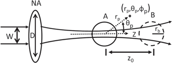
Figure 1. Any point in the image plane of the microscope objective is described in spherical coordinate by  . For this analysis the particle is placed at the focal point (position A) or away from the focal point by z0 (position B). The radius of the particle is rb.
Download figure:
Standard image High-resolution image3. Image plane formula
According to Richards and Wolf [20], the electric field Ei(rp, θp, ϕp) at any point in the image space if expressed in spherical coordinate is:

where I0, I1 and I2 are given by,
J0, J1, J2 are Bessel functions and ka is the medium wavenumber. θ is integrated to α, where α = sin−1(NA). F(θ) is the focusing function that we have added to the original formula to describe a collimated input Gaussian beam.
The focusing function F(θ) is given by [21],
The expression for I0, I1 and I2 given above is to be used when the focal spot coincide with the center of the particle. If the center of the particle is to be displaced from the center of the focal spot by z0, then simple change rpcos θp to rpcos θp + z0, with the origin at the particle's center.
It is noted that under paraxial conditions the focusing beam in the image space can be written as a series expansion with respect to the ratio of the beam waist versus diffraction length [22]. If only the first order term is retained then the focusing beam is Gaussian in shape. This Gaussian shape focusing beam at the particle position was used in reference [23] for calculating the nanojet formed by a dielectric particle. We use the Richard and Wolf formula [20] to describe the focusing beam. The input collimated beam before the microscope object is Gaussian, but the image field vector as describe by equations (1) and (2) in the focal region where the particle is located is not, in contrast with reference [23]. Furthermore, the Richard and Wolf formula is valid even for numerical aperture approaching one [24]. Using a microscope objective with NA = 0.85, the spatial profile of the focal spot predicted by the Richard and Wolf formula agreed very well with experimentally measured profile using a scanning NSOM probe [21].
4. Vector spherical harmonics analysis
The cos ϕp and/or sin ϕp dependence of Er, Eθ, Eϕ given above and the cos (mϕp) or sin (mϕp) dependence of the vector spherical harmonics given by (A2) in the appendix indicates that the only surviving expansion coefficients are Bo1n and Ae1n with m = 1 only. This conclusion is discussed in the appendix. Bo1n and Ae1n are calculated using equation (A12) which shows that Ae1n = −iBo1n. Therefore, the resultant incident field  expanded in vector spherical harmonics can be written as:

The superscript (0) indicates that the spherical Bessel function of the first kind jn is to be used. The coefficient En = Bo1n. Note that the form for the incident field  is exactly like the plane wave case except that coefficients which need to be calculated from (A12) are different.
It is necessary to determine the minimum number of summation terms needed in equation (4) so that  can faithfully recreates the expression for the exact incident field
  given by equation (1). For instance, the value of En is calculated using (A12) for a microscope objective with NA = 0.4 for medium focusing power, and 0.8 for strong focusing power. The collimated beam size is fixed at W = 2 mm, and objective's back focal plane aperture is fixed at D = 7.65 mm. Values of En that show the number of summation terms needed are given in table 1 in the appendix.
Table 1. Expansion coefficients En.
| NA = 0.4 | NA = 0.8 | |||
|---|---|---|---|---|
| n | En (10−3) | En (10−3) | ||
| Z0 = 0 | Z0 = 3.9 μm | Z0 = 0 | Z0 = 3.9 μm | |
| 1 | −147.7i | 46.906 + 96i | −0.086–591.3i | 125.90 + 82.09i |
| 2 | 79.44 | −52.88 + 24.74i | 285.28−0.03i | −47.61 + 67.92i |
| 3 | 53i | −15.98−36.54i | 161.85i | −45.36 − 35.20i |
| 4 | −38.4 | 27.66 − 11i | −94.70 − 0.02i | 28.81 − 32.70i |
| 5 | −28.86i | 7.702 + 21.98i | 0.03 − 55.00i | 24.24 + 24.90i |
| 6 | 22.14 | −17.95 + 5.307i | 31.37 + 0.03i | −22.65 + 18.31i |
| 7 | 17.13i | −3.49 − 14.89i | −0.03 + 17.54i | −12.99 − 20.20i |
| 8 | −13.3 | 12.45 − 2.078i | −9.67 − 0.03i | 18.49 − 8.86i |
| 9 | −10.27i | 0.974 + 10.43i | 0.02 − 5.22i | 5.33 + 16.88i |
| 10 | 7.9 | −8.71 + 0.115i | 2.73 + 0.02i | −15.21 + 2.29i |
| 11 | 6.04i | 0.538 − 7.232i | −0.01 + 1.34i | 0.30 − 13.42i |
| 12 | −4.57 | 5.94 + 1.016i | −0.60 − 0.01i | 11.48 + 2.44i |
| 13 | −3.43i | −1.35 + 4.82i | 0.01 − 0.25i | −4.14 + 9.43i |
| 14 | 2.56 | −3.83 − 1.55i | 0.12 + 0.01i | −7.29 − 5.36i |
| 15 | 1.88i | 1.64 − 2.98i | −0.01 + 0.09i | 6.08 − 5.15i |
| 16 | −1.37 | 2.26 + 1.65i | 3.06 + 6.31i | |
| 17 | −0.994i | −1.58 + 1.65i | −6.06 + 1.14i | |
| 18 | 0.716 | −1.143 − 1.465i | 0.54 − 5.39i | |
| 19 | 0.512i | 1.311 − 0.738i | 4.37 + 1.86i | |
| 20 | −0.365 | 0.422 + 1.137i | −2.75 + 3.13i | |
| 21 | −0.259i | −0.953 + 0.1844i | −1.80 − 3.17i | |
| 22 | 0.182 | −0.0158 − 0.7712i | 3.13 − 0.52i | |
| 23 | 0.126i | 0.601 + 0.0955i | −0.55 + 2.70i | |
| 24 | −0.086 | −0.16 + 0.448i | −1.98 − 1.33i | |
| 25 | −0.0566i | −0.136 − 0.1886i | 1.72 − 1.13i | |
| 26 | 0.035 | 0.1914 − 0.2072i | 0.31 + 1.91i | |
| 27 | 0.02i | 0.122 + 0.177i | −1.48 − 0.42i | |
| 28 | −0.1515 + 0.0595i | 0.88 − 0.98i | ||
| 29 | −0.0165 − 0.1213i | 0.40 + 1.06i | ||
| 30 | 0.091 + 0.0104i | −0.96 − 0.13i | ||
| 31 | −0.0236 + 0.0634i | 0.49 − 0.66i | ||
| 32 | −0.0398 − 0.0276i | 0.27 + 0.64i | ||
| 33 | 0.0259 − 0.0217i | −0.58 − 0.09i | ||
| 34 | 0.0093 + 0.0207i | 0.33 − 0.37i | ||
| 35 | −0.0142 + 0.001017i | 0.10 + 0.40i | ||
| 36 | 0.00352 − 0.0079i | −0.31 − 0.12i | ||
| 37 | 0.00261 + 0.00509i | 0.23 − 0.15i | ||
| 38 | −0.02 + 0.23i | |||
| 39 | −0.13 − 0.13i | |||
| 40 | 0.15 − 0.02i | |||
| 41 | −0.07 + 0.10i | |||
| 42 | −0.02 − 0.09i | |||
Figures 2(a') and (a) show the plot of  and
and  versus rp perpendicular to the optical axis
  and along the optical axis
  using the vector harmonics expansion of equation (4) and the Richard and Wolf formula of equation (1) respectively. The numerical aperture NA = 0.4. Figures 2(b') and (b) compare the same plot for NA = 0.8. If a sufficient number of summation terms is used, plots using equation (4) or equation (1) are indistinguishable as shown in figure 2, indicating that the vector harmonics expansion is a valid representation of the incident field.
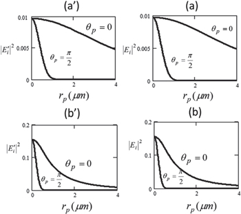
Figure 2. (a') and (a) compare the field intensity profile using the vector harmonic expansion formula and the Richard and Wolf formula respectively for NA = 0.4. (b') and (b) are the same comparison for NA = 0.8. θp = 0 is along the optical axis, and θp = π/2 is perpendicular to the optical axis, giving a focal spot size (FWHM) of 0.84 μm for NA = 0.4 and 0.42 μm for NA = 0.8.
Download figure:
Standard image High-resolution imageFor the case of the particle displaced from the focal plane by 3.9 μm, calculated coefficients  and the number of terms needed for both NA = 0.4 and 0.8 are also given in table 1 in the appendix. For NA = 0.4, figures 3(a') and (a) show the plot of
  and
and  versus rp for
  and
and  using the vector harmonic expansion and the Richard and Wolf formula respectively. The coordinate origin at rp = 0 is at the particle's center which is 3.9 μm away from the focal point. The FWHM of the beam spot size at the particle position is now 1.2 μm as indicated by the case corresponding to
  instead of 0.84 μm at the focal point. For the case corresponding to θp = π, the field intensity peaks at rp = 3.9 μm which is the focal point. Figures 3(b') and (b) show the same comparison plot for NA = 0.8. The field intensity at the coordinate origin at rp = 0, which is the position of the displaced particle center, is small because of the highly divergent beam for NA = 0.8. An expanded view of the field intensity for the case corresponding to
  shows the beam spot size at the particle position is 1.65 μm.
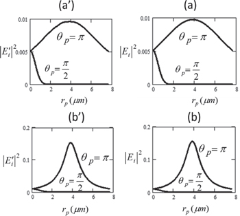
Figure 3. (a') shows the field intensity profile predicted by the vector harmonics expansion method if the coordinate rp = 0 is shifted 3.9 μm away from the focal point. (a) is the profile based on the Richard and Wolf formula. In figure (a') and (a), NA = 0.4. Figure (b') and (b) are the same comparison for NA = 0.8.
Download figure:
Standard image High-resolution imageWith the validity of the expansion of the incident field in terms of the vector harmonics established, we proceed to write the expression for the scattered field Ea and the field inside the particle Eb, which are given in (A16). Coefficients αan and βan etc are calculated from equation (A19–22). These coefficients are obtained by applying the boundary conditions for the tangential components of the electric and magnetic fields at r = rb, as given in (A15)
5. Nanojet calculations
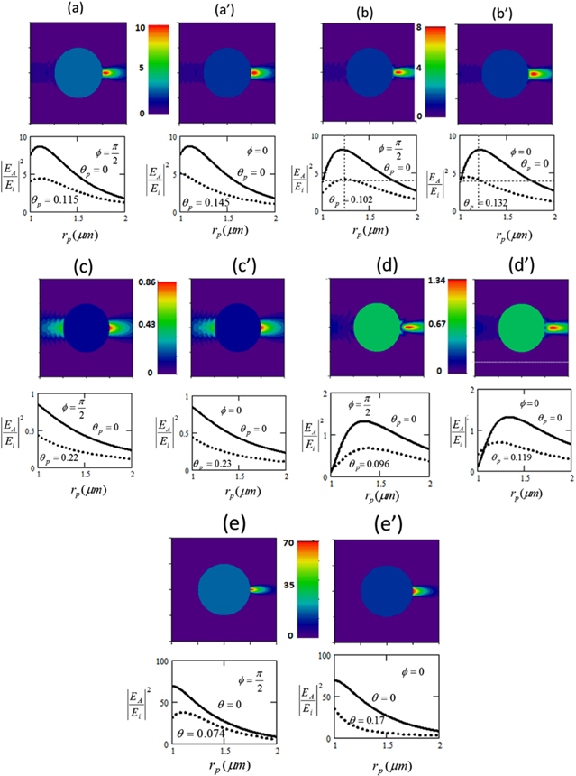
We present calculations of nanojets at a wavelength of 400 nm. The particle is assumed to be a fused silica particle with a diameter of 2 μm and a refractive index of 1.47 at 400 nm wavelength. Figures 4(a) and (a') show the nanojet formed when the focal point and the center of the particle are at the same point for the case corresponding to NA = 0.4. The width of the nanojet waist is a function of the azimuthal angle ϕ. Figure 4(a) is for the case  , which corresponds to the plane perpendicular to the plane formed by the incident electric field polarization and its propagation direction. The electric field intensity normalized to the focal intensity versus rp is shown below for θp = 0 and for θp = 0.115 when the intensity drops by one-half at the nanojet waist. From θp = 0.115, the calculated FWHM of the waist is about 253 nm. Figure 4(a') is for the case ϕ = 0, which correspond to the plane formed by the incident field polarization and its propagation direction. The half intensity occurs at θp = 0.145 as shown, which indicates that the FWHM of the waist is 319 nm. Figures 4(b) and (b') show the nanojet formed when the center of the particle is 3.9 μm away from the focal point. Compared with figures 4(a) and (a'), it is observed that the nanojet moved away from the surface of the particle by 215 nm. For ϕ = π/2, the half intensity occurs at θp = 0.102 which indicates that the FWHM of the waist is about 245 nm. For ϕ = 0, the FWHM is 316 nm. Thus the width of the waist remains about the same for the same ϕ but the position of the waist is moved farther outside the particle. Note that the nanojet field intensity is slightly smaller for figures 4(b) and (b') than for figures 4(a) and (a') because when the particle is displaced from the focal point, the FWHM of the incident beam at the particle is 1.2 μm rather than 0.84 μm; i.e. the particle collects less light. The asymmetry of the nanojet waist with respect to ϕ should be alleviated for circular polarization because the x or the y incident field polarization component is largely maintained during propagation.
Figure 4. The particle diameter is 2 μm with an index of 1.47. W = 2 mm, D = 7.65 mm. For (a) and (a'), the particle is at the focal point. For (b) and (b'), the particle is 3.9 μm from the focal point. NA = 0.4. Nanojet pictures are shown in the top diagram while the bottom diagrams show the normalized intensity as a function of rp for θp = 0 and for θp such that the intensity of the nanojet waist drops by 0.5. The intensity internal to the particle is not plotted but merely colored to show the position of the particle boundary with respect to the nanojet position. For (c) to (d'), the NA is 0.8. For (c), (c'), the particle is at the focal point while for (d) and (d') the particle is 3.9 μm away from the focal point. (e) and (e') are results for the plane wave case.
Download figure:
Standard image High-resolution image
Figures (c), (c'), (d), and (d') are cases when the NA = 0.8. For (c) and (c'), the particle is at the focal point. The nanojet waist is inside the particle. For (d) and (d'), the particle is 3.9 μm away from the focal point. The nanojet waist is now 335 nm outside the particle. For ϕ = π/2, the FWHM of the waist is 256 nm, and for ϕ = 0, it is 315 nm. Thus, the FWHM of the waist are roughly the same for NA = 0.4 and NA = 0.8.
In figures 4(e) and (e'), the result for the case of a plane wave incident field, as generally assumed, is also calculated and compared with the focused beam case. It is noted that for ϕ = π/2, the FWHM of the beam waist is as narrow as 150 nm and occurs at the surface of the particle. However, for ϕ = 0, the FWHM is 340 nm. Thus, the focused beam analysis produce a less asymmetric results compared with the plane wave analysis.
It is noted that nanojets intensity enhancement for focused beam shown in figures 4(a)–(d) are substantially smaller than for a plane wave beam shown in figure 4(e). This is reasonable because a nanoparticle collects much more photon for an incident focused beam than a plane wave, which theoretically is of infinite spatial extent. For instance, the intensity enhancement in figure 4(c) is only about one. If the enhancement were 100, the nanojet beam size would have to shrink to about 25 nm (factor of 10) since the definition of intensity is power/area.
6. Conclusion
We calculate nanojets formed by a focused incident beam instead of a plane wave. It is shown that the usage of vector spherical harmonics expansion of the focused beam allows a rigorous calculation of the 3D nanojets for two cases in which the particle's center is at or away from the focal point. We find that the position of the nanojet beam waist with respect to the particle surface can be positioned outside the particle by moving the particle's position away from the focal point with little change in the nanojet spot size. It is also found that for the case of a collimated linear polarized input beam focused by a microscope objective the nanojet spot size is more symmetric with respect to the azimuthal angle than the case when the incident field is a plane wave.
7. Appendix
The incident field Ei is expanded in terms of the orthogonal vector spherical harmonics as follows,
The full expression for the vector spherical harmonics Memn, Momn, Aemn, and Aomn as a function of spherical coordinates (rp, θp, ϕp) are listed in [25] equations (4)–(20):
Pnm(θp) is the associate Legendre function The radial function zn(ρ) is either the spherical Bessel function or the Hankel function ρ = krp, where k is the wavenumber. The orthogonal property between the vector spherical harmonics allows the coefficients such as, Bomn etc to be written as,
Contrast to reference [2, 19, 25], we provide an additional integration with respect to rp. To describe the field Ei at any point (rp, θp, ϕp) in the image space of a microscope objective, we use the formula given in reference [20] equations (2)–(32) with addition factors which are discussed below. If the input beam is polarized in the x-direction, then the focused incident field Ei on the particle in the image space of the objective are written in Cartesian coordinates [20] as:
Here, α, the limit of integration for θ is given by the numerical aperture NA of the microscope objective according to α = sin-1(NA). The additional factor F(θ) describes the specified microscope objective focusing of an incoming collimated Gaussian beam. F(θ) is given by [21].
where D is the diameter of the back focal aperture of the objective and W is the FWHM of the collimated incoming Gaussian beam (see figure 1). (A6) is not normalized with respect to the incident optical power, which is not an issue for calculations presented here.
Since the vector spherical harmonics are in spherical coordinates, it is necessary to transform Ei from Cartesian to spherical coordinates. Thus, unit vectors ex, ey and ez are transformed into unit vectors er, eθ, and eϕ in spherical coordinates according to familiar formulas, the results are:

With formulas given above and the numerical aperture of the microscope objective and the input beam parameters specified, it is shown that the focal spot spatial profile agrees very well with the measured profile using a NSOM tip in the collection mode of operation [21] If the focal plane is to be shifted away from the origin of the particle, then simply make the following change in the expression for I0, I1, and I2:

If z0 is positive, then the center of the particle at rp = 0 is to the right of the focal plane, which means that the beam is expanding at the particle's coordinate. If z0 is negative, the opposite is true.
Note that the ϕp dependence of all four vector harmonics in (A2) contains either cos(mϕp) or sin(mϕp) terms, whereas the ϕp dependence of Er, Eθ, Eϕ (A7) contains only cos ϕp or sin ϕp. Therefore, all expansion coefficients obtained from equation (A3) will be zero unless m = 1 since all coefficients are the product of vector harmonics and Ei. And ϕp is integrated from 0 to 2π. Moreover, with m = 1, coefficients Be1n involving Me1n and Ao1n involving No1n are zero because the integration over ϕp involving these terms are always the product of sin ϕp and cos ϕp which yields zero. Thus, the only non-zero coefficients in the expansion of Ei are Bo1n and Ae1n involving Mo1n and Ne1n respectively. We write  as,
as,

The superscripts (0) in the vector harmonics indicates that its radial components zn(ρ) are given by the spherical Bessel functions of the first kind jn(karp), where ka is the medium wavenumber. Expressions for the spherical vector harmonics Mo1n and Ne1n for the case m = 1, after conversion from the associated Legendre function P1n to the Legendre function Pn, are given as,
Here, y = cos θp. According to (A2), (A3) and (A7), Bo1n and Ae1n can eventually be written as
where jn(ρ) is the spherical Bessel funcion of order n, Pn(cos θp) is the Legendre function, y = cos θp, and I0, I1, and I2 are focal functions given in equation (A5)–(A6) with karp define as ρ. Numerical calculations using the formula given above yield Ae1n = −iBo1n like the plane wave case except that the value of Bo1n is different and changes with different degree of focusing. We define Bo1n as Bo1n ≡⃥ En, and rewrite  as
as

Denote the scattered electric and magnetic fields outside the particle as Ea and Ha. Inside the particle fields are denoted as Eb and Hb. When rp is outside the particle, the total field consists of the incident field plus the scattered field. Tangential components of the electric and magnetic fields in the eθ and eϕ direction must be equal at the particle-medium interface at rp = rb. This equality condition on E and H are expressed as:
Ei consists of a linear combination of Mo1n and Ne1n, therefore based on (A14) Ea and Eb are also a linear combination of Mo1n and Ne1n. Thus, Ea and Eb are expressed as
Since the scattered field resembles an outgoing wave, the appropriate general expression for zn describing the scattered field is the spherical Hankel function of the first kind: zn(ρp) = hn(karp), with hn(ρp) ≡⃥ jn(ρp) + i yn(ρp), where yn(ρp) is the spherical Bessel function of the second kind. The superscript (1) indicates the usage of this spherical Hankel function of the first kind.
To describe the field inside the particle zn(ρp) = jn(kbrp) since jn does not diverge at the origin. Here, kb is the wavenumber associated with the particle.
The magnetic field Hi, Ha, Hb can be obtained from

Using the relationship between the vector harmonics N and M as given by reference [25], H are written as
with (A14) and (A16) and (A18) inserted into the boundary conditions, (A15) at rp = rb, one obtains four equations that solve for the four constants αan, αbn, βan, βbn. They are in determinate form,
with αan, αbn, βan, βbn calculated and En obtained from (A16) for the case of the focused beam, all electric and magnetic fields as a function of (rp, θp, ϕp) are given.