
Abstract
The propagation of Dyakonov–Tamm waves guided by the planar interface of an isotropic topological insulator and a structurally chiral material, both assumed to be nonmagnetic, was investigated by numerically solving the associated canonical boundary-value problem. The topologically insulating surface states of the topological insulator were quantitated via a surface admittance  , which significantly affects the phase speeds and the spatial profiles of the Dyakonov–Tamm waves. Most significantly, it is possible that a Dyakonov–Tamm wave propagates co-parallel to a vector
  in the interface plane, but no Dyakonov–Tamm wave propagates anti-parallel to
  . The left/right asymmetry, which vanishes for
  , is highly attractive for one-way on-chip optical communication.
Export citation and abstract BibTeX RIS

Original content from this work may be used under the terms of the Creative Commons Attribution 3.0 licence. Any further distribution of this work must maintain attribution to the author(s) and the title of the work, journal citation and DOI.
1. Introduction
Dyakonov–Tamm waves are electromagnetic surface waves whose propagation is guided by the planar interface of two dielectric materials, one of which is isotropic and homogeneous whereas the second is anisotropic and periodically nonhomogeneous normal to the interface plane [1]. In contrast, the second partnering material must be isotropic for Tamm-wave propagation [2–5], whereas that material must be homogeneous for Dyakonov-wave propagation [6–8]. All three types of surface waves propagate ideally without attenuation, unlike surface-plasmon-polariton waves [9], as all three exist in all-dielectric metamaterial architectures [10]. Dyakonov and Dyakonov–Tamm waves offer different phase speeds in different directions of propagation in the interface plane, which makes them more attractive than Tamm waves for communication. But, while the allowed directions of propagation of Dyakonov waves are confined to two minute angular sectors (typically, each less than 1° in width [8, 11]) in the interface plane, Dyakonov–Tamm waves were theoretically predicted not to suffer from that restriction. The existence of these waves has been confirmed recently in two distinct experimental configurations [12, 13].
Theoretical investigation [14] has recently shown that left/right asymmetry can be introduced in Dyakonov-wave propagation by
- (i)
- (ii)choosing the anisotropic, homogeneous, dielectric partnering material to possess orthorhombic crystallographic symmetry such that no more than one of the three eigenvectors of its relative permittivity dyadic lies in the interface plane.
Then, the Dyakonov wave propagating coparallel to a vector  in the interface plane has a different phase speed and different spatial profile as compared to the Dyakonov wave which propagates antiparallel to
  . Indeed, it may be possible for a Dyakonov wave to propagate coparallel to
  but for no Dyakonov to propagate antiparallel to
  . We refer to this asymmetry with respect to interchanging the direction of surface-wave propagation as left/right asymmetry. The exploitation of left/right asymmetry is promising for one-way optical devices, which could reduce backscattering noise [18] in optical communication networks, microscopy, and tomography, for example. Let us note here that left/right asymmetry is not exhibited when the TISS are replaced by ordinary surface conducting states [19, 20].
Although the incorporation of an isotropic topological insulator (TI) as a partnering material [16, 21] introduces left/right asymmetry in surface-wave propagation, the angular sectors of allowable propagation remain minute in extent [14]. With the aim of widening those angular sectors, we decided to make the anisotropic partnering material periodically nonhomogeneous in the direction normal to the interface plane. Specifically, we chose that partnering material to be a structurally chiral material (SCM) [1]—exemplified by chiral smectic liquid crystals [22] and chiral sculptured thin films [23]—the other partnering material being an isotropic TI [24, 25].
The plan of this paper is as follows. Section 2 contains a formulation of the canonical problem for Dyakonov–Tamm-wave propagation guided by the planar interface of an isotropic TI and an SCM. In the canonical problem, all space is partitioned into two half spaces, one of which is occupied by one partnering material and the second by the other partnering material. Although practically unimplementable in the strict sense, the canonical problem lies at the heart of practically implementable configurations such as the prism-coupled, grating-coupled, and waveguide-coupled configurations [26, 27]. Numerical results are provided and discussed in section 3.
An  dependence on time t is implicit, with ω denoting the angular frequency and
  . The free-space wavenumber, the free-space wavelength, and the intrinsic impedance of free space are denoted by
  ,
,  , and
, and  , respectively, with
  and
and  being the permeability and permittivity of free space. The speed of light in free space is denoted by
  . Vectors are in boldface; dyadics are underlined twice; Cartesian unit vectors are identified as
 and
and  column vectors are in boldface and enclosed with square brackets; and matrixes are underlined twice and enclosed with square brackets.
2. Theory
A schematic of the boundary-value problem for the propagation of the Dyakonov–Tamm wave is provided in figure 1. The half-space  is occupied by an isotropic TI with a relative permittivity
  and a surface admittance
  which quantifies the TISS [16] that arise in consequence of a geometric phase that cannot be gauged away in a cyclic system [28, 29]. Alternatively, the half-space
  can be modeled as being occupied by an isotropic, nonreciprocal, achiral, nonmagnetic material with relative permittivity
  and Tellegen parameter
  but we prefer the former description because it brings out the presence of TISS very clearly [20] and conforms to the Post constraint [21].

Figure 1. Schematic of the boundary-value problem solved.
Download figure:
Standard image High-resolution imageThe half-space  is occupied by an SCM whose permittivity dyadic is given by

Here, the dyadics
h = 1 for structural right-handedness and  for structural left-handedness;
  is the structural period of the SCM along the z axis; and
 ![$\chi \in (0,\pi /2]$](https://content.cld.iop.org/journals/2040-8986/18/11/115101/revision1/joptaa3c62ieqn29.gif) . Whereas
. Whereas  and
and  for cholesteric liquid crystals,
  and
and ![$\chi \in (0,\pi /2]$](https://content.cld.iop.org/journals/2040-8986/18/11/115101/revision1/joptaa3c62ieqn33.gif) for chiral smectic liquid crystals [22] and chiral sculptured thin films [23]. Both partnering materials are assumed to be nonmagnetic.
for chiral smectic liquid crystals [22] and chiral sculptured thin films [23]. Both partnering materials are assumed to be nonmagnetic.
2.1. Field representations
We consider the Dyakonov–Tamm wave to be propagating parallel to the unit vector  ,
,  , in the xy plane and decaying far away from the interface z = 0. With q as the wavenumber of the Dyakonov–Tamm wave, the electric and magnetic phasors can be represented everywhere by

In the region  , the field phasors may be written as [21, 27]
and
where A1 and A2 are unknown scalars, q is positive and real-valued for unattenuated propagation in the xy plane,  , and
, and  for attenuation as z→ −
 .
.
The field representation in the region  requires the formulation of the column vector [23, 27]

which satisfies the matrix differential equation [1]

where the 4 × 4 matrix
and the scalar

Equation (7) has to be solved numerically in order to determine the matrix ![$[\underline{\underline{Q}}]$](https://content.cld.iop.org/journals/2040-8986/18/11/115101/revision1/joptaa3c62ieqn41.gif) that appears in the relation
that appears in the relation

to characterize the optical response of one period of the SCM.
By virtue of the Floquet theory [30], we can define a matrix ![$[\underline{\underline{\tilde{Q}}}]$](https://content.cld.iop.org/journals/2040-8986/18/11/115101/revision1/joptaa3c62ieqn42.gif) such that
such that

Both ![$[\underline{\underline{Q}}]$](https://content.cld.iop.org/journals/2040-8986/18/11/115101/revision1/joptaa3c62ieqn43.gif) and
and ![$[\underline{\underline{\tilde{Q}}}]$](https://content.cld.iop.org/journals/2040-8986/18/11/115101/revision1/joptaa3c62ieqn44.gif) share the same eigenvectors, and their eigenvalues are also related. Let
share the same eigenvectors, and their eigenvalues are also related. Let ![${[{\bf{t}}]}^{(n)}$](https://content.cld.iop.org/journals/2040-8986/18/11/115101/revision1/joptaa3c62ieqn45.gif) ,
,  , be the eigenvector corresponding to the nth eigenvalue
  of
of ![$[\underline{\underline{Q}}];$](https://content.cld.iop.org/journals/2040-8986/18/11/115101/revision1/joptaa3c62ieqn48.gif) then, the corresponding eigenvalue
then, the corresponding eigenvalue  of
of ![$[\underline{\underline{\tilde{Q}}}]$](https://content.cld.iop.org/journals/2040-8986/18/11/115101/revision1/joptaa3c62ieqn50.gif) is given by
is given by

2.2. Dispersion equation
For the Dyakonov–Tamm wave to propagate parallel to  we must ensure that
  , and set

where B1 and B2 are unknown scalars, and ![$[{\bf{f}}({z}^{\pm })]$](https://content.cld.iop.org/journals/2040-8986/18/11/115101/revision1/joptaa3c62ieqn53.gif) stands for
stands for ![${{\rm{lim}}}_{\delta \to 0}\,[{\bf{f}}(z\pm \delta )]$](https://content.cld.iop.org/journals/2040-8986/18/11/115101/revision1/joptaa3c62ieqn54.gif) with
with  . The other two eigenvalues of
 ![$[\underline{\underline{\tilde{Q}}}]$](https://content.cld.iop.org/journals/2040-8986/18/11/115101/revision1/joptaa3c62ieqn56.gif) describe waves that amplify as
describe waves that amplify as  and cannot therefore contribute to the Dyakonov–Tamm wave. At the same time
by virtue of equations (4) and (5).
Whereas the tangential component of the electric field phasor is continuous across the plane z = 0, the existence of the protected TISS on the boundary of the TI implies a discontinuity in the tangential component of the magnetic field phasor across the same plane [14, 20, 21]. Accordingly
which may be rearranged as

For a nontrivial solution, the 4 × 4 matrix ![$[\underline{\underline{M}}]$](https://content.cld.iop.org/journals/2040-8986/18/11/115101/revision1/joptaa3c62ieqn58.gif) must be singular, so that
must be singular, so that

is the dispersion equation for the Dyakonov–Tamm wave.
3. Numerical results and discussion
We numerically solved the dispersion equation to obtain the normalized wavenumbers  of the Dyakonov–Tamm waves. Knowing q, we can calculate the phase speed
  of the Dyakonov–Tamm wave. The spatial profile of the rate of energy flow associated with a Dyakonov–Tamm wave is provided via the time-averaged Poynting vector
 ![${\bf{P}}({\bf{r}})\equiv {\bf{P}}(x,y,z)=(1/2){\rm{Re}}[{\bf{e}}(z)\times {{\bf{h}}}^{* }(z)]$](https://content.cld.iop.org/journals/2040-8986/18/11/115101/revision1/joptaa3c62ieqn61.gif) , where the asterisk denotes the complex conjugate.
, where the asterisk denotes the complex conjugate.
For all numerical results reported here, we fixed  and
and  . For definiteness, the SCM was taken to be a chiral sculptured thin film, which comprises an array of parallel nanohelixes that rise at an angle χ to the interface plane by means of a vapor deposition process [23]. In accordance with empirical relationships determined for a columnar thin film of patinal titanium oxide produced by directing the vapor flux at an angle
  onto a rotating substrate, the principal relative permittivities are [31]
with  being in degree, and the angle

We considered  along with
  , but kept
  variable, where
  is the fine structure constant [32]. The direction of propagation was also varied in the xy plane, i.e.,
  . All calculations were restricted to
  to avoid computational instabilities that emerged for
  , whereas
  must be greater than
  to ensure that
  .
.
In figure 2(a),  is displayed as a function of both ψ and
  when
when  and
and  . Solutions to the dispersion equation (17) were found in the range
  corresponding to a normalized phase speed
  in the range
  . Dyakonov–Tamm-wave propagation is exhibited for
 ![$\psi \subseteq [0^\circ ,16^\circ ]\cup [92^\circ ,196^\circ ]\ \cup [272^\circ ,360^\circ ]$](https://content.cld.iop.org/journals/2040-8986/18/11/115101/revision1/joptaa3c62ieqn83.gif) , the widths of the angular sectors available for Dyakonov–Tamm-wave propagation being large in comparison to the
, the widths of the angular sectors available for Dyakonov–Tamm-wave propagation being large in comparison to the  widths of angular sectors for Dyakonov-wave propagation [14].
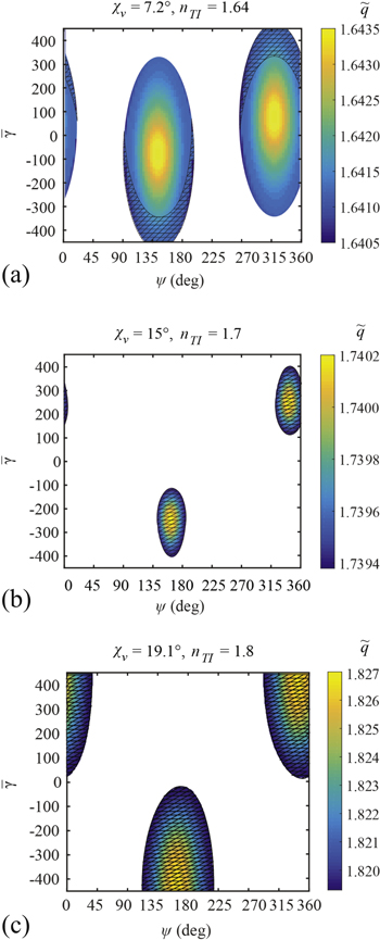
Figure 2.
 as a function of both ψ and
  for (a)
  ,
,  (b)
(b)  ,
,  and (c)
  ,
,  . Cross hatching identifies those values of ψ for which a Dyakonov–Tamm wave exists but does not exist for
  . Blank areas: no solution of equation (17).
Download figure:
Standard image High-resolution imageThe same is true in figure 2(b) for  and
and  , and in figure 2(c) for
  and
and  . In figure 2(b), the solutions cover the range
  , corresponding to normalized phase speeds in the range
  . In figure 2(c), the solutions cover the range
  , corresponding to normalized phase speeds in the range
  .
.
All three panels in figure 2 indicate that the propagation of Dyakonov–Tamm waves, if it can occur for chosen values of the pair  , is possible in two non-overlapping regions in the
  plane. Each region is bounded by an elliptical contour represented parametrically as the ellipse
  , with
The region described by  is located roughly in the center of the
  plane in each panel, while the region described by
  is split into two parts because
  is cyclic with period 360°. The center of the ellipse is located at
  for
for  , the projection of each ellipse on the ψ axis is
  , and the projection of each ellipse on the
  axis is
  . Values of the parameters
  and
and  for all three panels are provided in table 1.
Table 1.
Parameters in equation (20) delineating the regions in the  plane in which the propagation of Dyakonov–Tamm waves is allowed in figures 2(a)–(c).
| Figure 2 |

|

|

|

|

|

|
|---|---|---|---|---|---|---|
| (a) | 7.2° | 1.64 | −38° | 52° | 80 | 450 |
| (b) | 15.0° | 1.70 | −18° | 21° | 248 | 145 |
| (c) | 19.1° | 1.80 | −16° | 53° | 415 | 395 |
Figure 2 clearly shows that Dyakonov–Tamm waves are allowed for both positive and negative values of the surface admittance  . However, the angular sectors (on the ψ axis) are different for
  than for
  .
.
Whereas Dyakonov–Tamm-wave propagation is possible for  in figure 2(a), that is not true in figures 2(b) and (c). Therefore, the incorporation of the protected TISS with an appropriate value of
  can trigger the excitation of Dyakonov–Tamm waves.
Left/right asymmetry is evident in all three panels in figure 2. If Dyakonov–Tamm waves are allowed to propagate in the two directions indicated by ![$\psi \in [0^\circ ,180^\circ ]$](https://content.cld.iop.org/journals/2040-8986/18/11/115101/revision1/joptaa3c62ieqn128.gif) and
and  for a specific value of
  , the two Dyakonov–Tamm waves have different phase speeds (and, therefore, other characteristics). More significantly, figure 2 makes it clear that if a Dyakonov–Tamm wave can propagate in the direction indicated by
  ), there is also the likelihood that no Dyakonov–Tamm wave can propagate in the direction indicated by
  . Cross hatching in all three panels highlights the values of ψ for which Dyakonov–Tamm-wave propagation is possible but not for
  . These regions of total left/right asymmetry are very attractive for one-way devices, although they require high values of
  [17].
[17].
Further insights into the nature of these Dyakonov–Tamm waves may be gained by considering the spatial profiles of the Cartesian components of the electric and magnetic field phasors, along with those of the corresponding time-averaged Poynting vector. To allow for a consistent comparison, the amplitude of the time-averaged Poynting vector was constrained as  W m−2. Then, by virtue of equations (4) and (5), we get

which allows all coefficients in the column vector on the left side of equation (16) to be specified.
The Cartesian components of  are plotted versus z in figure 3 for the Dyakonov–Tamm wave excited when
  ,
,  , and
, and  . A comparison of figures 3(a) and (b) reveals that, for
  , the power density is slightly more confined to the TI when
  is positive while for negative
  the confinement is slightly greater to the SCM. In contrast, a comparison of figures 3(c) and (d) reveals that, for
  , the power density is slightly more confined to the TI for negative
  while the confinement is slightly greater to the SCM for positive
  . After noting that
  , left/right asymmetry becomes evident on comparing figures 3(a) and (c) and/or comparing figures 3(b) and (d). The signs of Px and Py are reversed when together
  changes to
  and
and  changes to
  , as may be appreciated after comparing figures 3(b) and (c) and/or comparing figures 3(a) and (d).
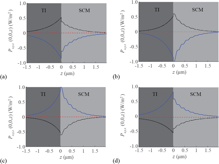
Figure 3. Spatial variations of the Cartesian components of the time-averaged Poynting vector  of the Dyakonov–Tamm wave guided by the TI/SCM interface when
  and
and  . (a)
. (a)  and
and  , (b)
, (b)  and
and  , (c)
, (c)  and
and  , (d)
, (d)  and
and  . The components parallel to
 and
and  are represented by blue solid, black broken dashed, and red dashed lines, respectively.
Download figure:
Standard image High-resolution imageFigures 4 and 5 show the magnitudes of the Cartesian components of  and
and  respectively, plotted against z for the same values of
  ,
,  ψ, and
  as used for figure 3. All Cartesian components decay exponentially inside the TI as z→ −
 , consistently with equations (4) and (5). The periodic undulations of the Cartesian components inside the SCM dampen as
  , in accord with the periodic nonhomogeneity of the SCM [27], as is warranted by Floquet theory [30].

Figure 4. Same as figure 3 except that the magnitudes of the Cartesian components of the electric field phasor  are plotted.
Download figure:
Standard image High-resolution image
Figure 5. Same as figure 3 except that the magnitudes of the Cartesian components of the magnetic field phasor  are plotted.
Download figure:
Standard image High-resolution imageThe spatial profiles of the Cartesian components of the electric and magnetic field phasors in figures 4 and 5 vary relatively little in the SCM when either  changes to
  or
or  changes to
  , but more substantial variations are observed in the TI, especially for Ez, Hx, and Hy. Left/right asymmetry is obvious, e.g., on comparing figures 4(a) and (c) or comparing figures 5(b) and (d). Finally, the spatial profiles of the fields remain unchanged when
  changes to
  and
and  changes to
  , as may be appreciated by comparing figures 4(b) and (c) and/or comparing figures 5(a) and (d).
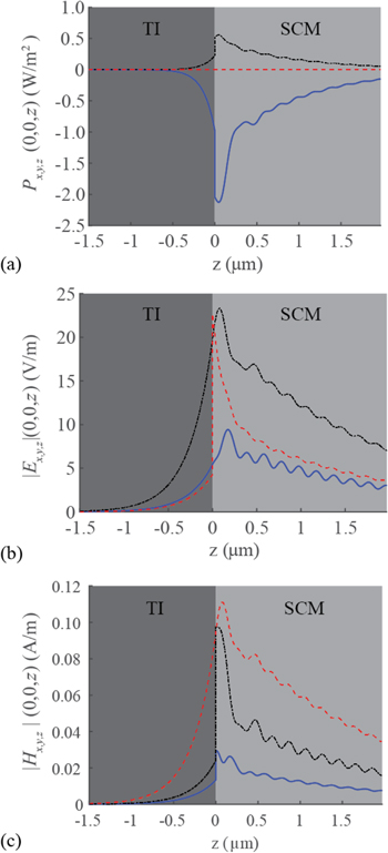
Similar conclusions can be drawn looking at the spatial profiles for a case of total left/right asymmetry, in which Dyakonov–Tamm-wave propagation is possible for some ψ but not for  . As an example, figure 6 provides the spatial profiles of magnitudes of the Cartesian components of
  ,
,  , and
, and  of the Dyakonov–Tamm wave guided by the TI/SCM interface when
  ,
,  ,
,  , and
, and  . Dyakonov-wave propagation is not possible for
  , other parameters remaining unchanged, according to figure 2(b). The spatial profiles in figure 6 are very similar to those in figures 3(b), 4(b), and 5(b), for which
  and
and  .
.
Figure 6. Spatial variations of the Cartesian components of (a)  , (b)
, (b)  , and (c)
  of the Dyakonov–Tamm wave guided by the TI/SCM interface when
  ,
,  ,
,  , and
, and  . The components parallel to
 and
and  are represented by blue solid, black broken dashed, and red dashed lines, respectively.
Download figure:
Standard image High-resolution image
A discussion of the discontinuities and continuities of the Cartesian components of the electric and magnetic field phasors across the plane z = 0 is in order. Both Ex and Ey must be continuous while Ez must be discontinuous, according to the standard boundary conditions of electromagnetics [33]. The plots in figures 4 and 6(b) are in accord with these constraints. As both partnering materials have been taken to be non-magnetic, Hz must be continuous across the plane z = 0 [33]. The plots in figures 5 and 6(c) show this continuity. The existence of the protected TISS must make Hx and Hy discontinuous across the plane z = 0, which is evident in figures 5 and 6(c). The continuities of Ex and Ey and the discontinuities of Hx and Hy were, of course, incorporated via equation (15).
4. Concluding remarks
We formulated and solved the boundary-value problem for electromagnetic surface waves guided by the planar interface of an SCM and a TI, both materials assumed to be nonmagnetic. The protected TISS on the interface were quantitated through a surface admittance  . Our numerical investigation demonstrated that the phase speeds and the spatial profiles of Dyakonov–Tamm waves are significantly affected by
  . A left/right asymmetry is exhibited whereby the phase speed and electromagnetic field profiles for a Dyakonov–Tamm wave that propagates co-parallel to a vector
  in the interface plane are generally different to those for a Dyakonov–Tamm wave that propagates anti-parallel to
  . Even more importantly, the existence of a Dyakonov–Tamm wave that propagates co-parallel to a vector
  in the interface plane does not imply the existence of a Dyakonov–Tamm wave that propagates anti-parallel to
  . The left/right asymmetry, which vanishes if the surface admittance vanishes, is highly attractive for one-way on-chip optical communication.
Acknowledgments
TGM acknowledges the support of EPSRC Grant EP/M018075/1. A Lakhtakia thanks the Charles Godfrey Binder Endowment at the Pennsylvania State University for ongoing support of his research.