


ABSTRACT
We report on the analysis of subsurface vorticity/helicity measurements for flare producing and quiet active regions. We have developed a parameter to investigate whether large, decreasing kinetic helicity density commonly occurs prior to active region flaring. This new parameter is effective at separating flaring and non-flaring active regions and even separates among C-, M-, and X-class flare producing regions. In addition, this parameter provides advance notice of flare occurrence, as it increases 2–3 days before the flare occurs. These results are striking on an average basis, though on an individual basis there is still considerable overlap between flare associated and non-flare associated values. We propose the following qualitative scenario for flare production: subsurface rotational kinetic energy twists the magnetic field lines into an unstable configuration, resulting in explosive reconnection and a flare.
Export citation and abstract BibTeX RIS
1. INTRODUCTION
As our society becomes more technologically advanced, space weather is an increasing concern. Solar flares and coronal mass ejections (CMEs) affect satellite function, high-frequency communication, and power grids, as well as many applications related to GPS (e.g., deep-sea drilling and precision farming). Because of our increasing reliance on technology that is very susceptible to space weather effects, it is vital that we improve our understanding of solar flares and increase our ability to forecast when a flare will occur and how large it will be.
Highly twisted magnetic fields are very likely responsible for strong eruptive phenomena such as flares and CMEs. For example, Falconer et al. (2009) have shown that flare-productive active regions are located on a straight line in a phase-space diagram of the total free energy of the magnetic field and the total magnetic flux. The input of free energy via convection in and below the photosphere balances the loss of free energy via CMEs and flares. Currently, several parameters based on surface magnetic field measurements are being evaluated as potential flare-forecasting criteria (see, for example, Georgoulis & Rust 2007; Leka & Barnes 2007; Schrijver 2007).
In this Letter, we look at the contribution of twisted magnetic fields below the surface of the Sun to flare production. These field motions can be measured indirectly through the use of local helioseismology using the ring diagram technique (Hill 1988; Haber et al. 2002). In this technique, localized regions are probed rather than the entire Sun, making it possible to map the horizontal flows in the outer convection zone as a function of heliographic latitude, longitude, depth, and time. This technique has led to detailed maps of the horizontal flows, with continual coverage since 2001 August using data from the Global Oscillation Network Group (GONG) program. The 100+ Carrington rotations that have been collected so far cover solar maximum and the descending phase of cycle 23, as well as the current extended and deep minimum.
While the flow maps themselves are a rich source of information about the solar convection zone, their value is enhanced by the computation of fluid dynamics descriptors, such as the divergence and the vorticity of the flows. Vertical velocities are determined using the divergence of the horizontal flows, assuming incompressible flows and zero surface velocity (reasonable given the size and timescales involved). The kinetic helicity density is then the scalar product of the velocity and vorticity vector. See Komm (2007) for additional details. In the remainder of this Letter, we use the shorthand term "helicity" to denote "kinetic helicity density."
Komm et al. (2004) showed that the helicity of AR10486 had very large values that shrank to essentially zero at the point when an X10 flare occurred. In this Letter, we investigate 1023 active regions to determine if this behavior is typical or if AR10486 was unusual. We derive a parameter to capture the large but shrinking helicity, and we show that this parameter effectively indicates 2–3 days in advance if a given active region will produce a flare and approximately how large it will be.
2. DATA ANALYSIS
Starting with the GONG one-per-minute full-disk Doppler velocity images, we split the solar surface into 189 overlapping regions, each with a 15° diameter and with centers spaced by 7 5. The areas cover the disk out to ±525 in both latitude and central meridian distance. Each region is remapped to remove the foreshortening caused by the spherical surface of the Sun and is tracked at approximately the surface rotation rate for a period of 1664 minutes (approximately 1 day). This method is further described in Komm et al. (2004). This data set consists of 1023 active regions with each active region having 7–8 days of data. Helicity is determined at 16 different depths (ranging from 0.6 Mm to 15.8 Mm). For each individual measurement, we have total helicity, as well as the vorticity magnitude and components in the x-, y-, and z-direction. Flare magnitudes, times, and associated active regions are available on the NGDC Web site (http://www.ngdc.noaa.gov/stp/SOLAR/ftpsolarflares.html).
In Figure 1, we take all active regions associated with 250 M-class flares and 40 X-class flares and plot the average helicity values as a function of time from the flare for each of the 16 depths. To produce this plot (commonly called a superposed epoch analysis) for each event, we center the data in time on the day of the flare and average the values of helicity. The resulting plot shows the average values at each depth as a function of time to the flare initiation. Error bars indicate the standard error of the mean, i.e.,  where σ is the standard deviation of the data and n is the number of points. The curves for each depth are slightly offset horizontally from one another to avoid merging of the error bars. As there are a maximum of 8 days of data for each active region, the superposed epoch analysis ranges from −7 to 6 days (in Figure 1 only days −6 to 2 are shown).
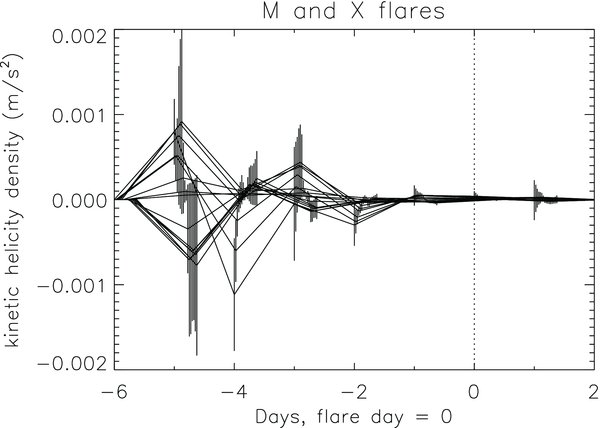
Figure 1. Average helicity values for each depth as a function of days to flare. Each curve corresponds to a different depth and is composed of the average of 290 active regions, 250 associated with an M-class flare and 40 associated with an X-class flare.
Download figure:
Standard image High-resolution imageIf there are multiple flares from the same active region, the high values from the previous flare can affect the pre-event values of the current flare. To reduce this effect, we include at least 2 days after each flare in the calculation for that event and exclude those data from the calculations for any following events. Each subsequent data point is considered to belong to the next flare. This method is used for all of the data presented in this Letter. For cases in which flare magnitudes are considered separately (Figures 2–4), larger flares are given precedence (i.e., data from an X-class flare that occurs a day after an M-class flare will appear in the X-class flare results, while that M-class flare will be ignored in the analysis).
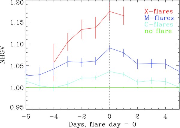
Figure 2. Superposed epoch analysis for active regions associated with X-class flares (red), M-class flares (blue), and C-class flares (cyan). Shown in green is an average value for active regions that do not flare.
Download figure:
Standard image High-resolution image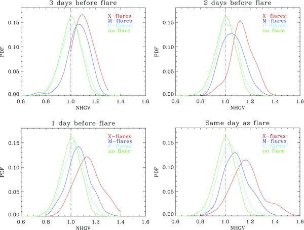
Figure 3. Probability density functions for active regions that produce an X-class, M-class, C-class or no flare. The panels indicate the distributions at different times relative to the flare occurrence.
Download figure:
Standard image High-resolution image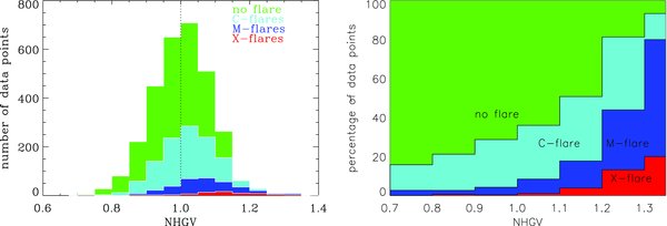
Figure 4. Histogram of NHGV values in number of events (left) and as a percentage of the total (right). Events with no associated flares (green) dominate. Values for non-flaring active regions are shifted to lower NHGV values compared to the rest of the distribution.
Download figure:
Standard image High-resolution image
Figure 1 has a similar character to the single event shown in Komm et al. (2004), with helicity values initially having a large spread in values with depth that gradually decreases to zero for all depths at the time of the flare, suggesting that subsurface helicity plays some role in flare production. To capture this information in a single variable, we first calculate quiet spectra for each depth based on 980 quiet Sun regions and normalize by dividing the value at each depth by the average quiet value at each depth. Similarly, observational differences across the solar disk are accounted for by dividing by the average quiet value at each position on the Sun. At this point, we have the helicity as a function of depth (z) and time (t). We take the difference in helicity at each depth from one day to the next to capture the shrinking values seen in Figure 1 (Δhz(t) = hz(t) − hz(t − 1)). In order to determine the spread of this temporal helicity change with depth, we sum the change in Δhz with depth (Δh(t) = Σz(Δhz(t) − Δhz − 1(t))). This parameter, Δh, captures the large, but shrinking, spread of helicity changes at time t. We then, separately, sum the change in helicity with depth (h(t) = Σz(hz(t) − hz−1(t)), capturing the overall spread of helicity values. We multiply these two quantities together and call the total parameter the Normalized Helicity Gradient Variance (NHGV). For the average event seen in Figure 1, this parameter should capture the large, shrinking values leading up to the flare.
In Figure 2, we plot a superposed epoch analysis of all flaring active regions using the same technique described for Figure 1. Here we plot NHGV versus time, and we normalize these data based on quiet, non-flaring active regions. The error bars are the standard error of the mean, as described above. As there is no "time to flare" for the non-flaring active regions, there is just one average value for "quiet" regions. The normalization produces a value of 1 for quiet regions that is shown in green. It is immediately apparent that the NHGV parameter is able to separate among flare classes with C-, M-, and X-class flare producing active regions having NHGV values that increase with increasing flare class and all of these values are higher than the ambient quiet region data. This increase with flare class is consistent with previous associations between helicity and flare value (Mason et al. 2006; Komm & Hill 2009). This parameter rises in the days before the flare occurs, peaking on the day of the flare. A statistically significant jump in NHGV is seen 2 days before C and X-class flares and 3 days before M-class flares. Though this result is based on averaged data, it indicates the potential ability to use these data to predict when a flare will occur (within 24 hr), how large it will be (order of magnitude, i.e., C-, M-, or X-class), and which active region it will arise from.
In Figure 3, we plot probability distribution functions (PDFs) of the NHGV value for each flare class and for regions that do not produce a flare in the specified time period. In the top left hand panel, we plot PDFs for active regions that will produce a flare in 3 days. The C-class flare distribution is only slightly offset from the quiet distribution, while the M- and X-class distributions skew to larger values of NHGV with peaks of 7% and 9% above the mean quiet value and tails that reach up to 30% higher than the mean quiet value. In the top right hand panel, we plot the NHGV distribution 2 days before the flare. Here, the C- and M-class flare distributions are slightly offset from quiet values, peaking at about 5% with the tail of the M-class flare distribution reaching to larger values, while the X-class flare distribution peaks at 12% above the quiet mean. In the bottom left hand figure, 1 day prior to the flare, the distributions for X-class flares, M-class flares, C-class flares, and quiet regions are centered on progressively smaller values. The same is true on the day of the flare, with the X-class flare distribution peaking at 20% and extending to nearly 60% above the ambient mean. These populations overlap, but are distinct, with larger NHGV values for larger flares. In addition, there is a temporal progression with higher NHGV values occurring at time periods closer to the flare initiation.
In Figure 4 (left), we plot the distribution of NHGV with flare size in histogram form for all data within 3 days before and including the day of the flare. Events without an associated flare (green) represent the largest population of data. The distribution of the NHGV value for these events is centered on 1.0, and the C-class (cyan), M-class (blue), and X-class (red) flares trend to larger values of NHGV as can also be seen in Figure 3. In this plot, we see the main challenge in this (or any other) method for flare predictions: the very small number of X- and M-class flares. Though larger values of NHGV are associated with larger flares, the tail of the non-flaring distribution overlaps these high NHGV values. However, we again see that the distribution of NHGV differs for flaring versus non-flaring active regions. The distribution for flare-associated events is offset slightly to increasingly higher values of NHGV. We calculate whether flare-associated and non-flare-associated NHGV values come from the same population using the Kolmogorov–Smirnov statistic (Press et al. 1989). We compare all NHGV values within 3 days prior to a flare of C-class or above with NHGV values for active regions that do not flare. We find a value of 0.19, indicating that the probability of flaring and non-flaring active region NHGV values coming from the same population is 2.3e-33. It is clear that flare/non-flare populations are distinct.
In the right panel of Figure 4, we plot the same data in terms of percentage of events at each value rather than the total number of events. We see more clearly in this figure that the percentage of large flare-associated events increases with increasing NHGV. At a value of NHGV of 1.1 there is a 50% chance of at least a C-class flare, while beyond 1.2 more than 80% of all periods are flare associated. Below a value of 1, there is only a 20% chance that the active region will flare and only a 3% chance that the active region will produce an M- or X-class flare.
Using the discriminant analysis technique (Leka & Barnes 2007), we have combined NHGV with the surface magnetic field to determine their predictive value. To obtain the surface magnetic field, we average 96 minute Michelson Doppler Imager magnetograms over the length of a ring day and bin them into circular areas to match the size of the ring-diagram patches (for details, see, Komm et al. 2009). We have found that the combination of the temporal evolution of NHGV and the surface magnetic field strength provides a flare versus no-flare forecast within 1 day of a flare with a Heidke skill score of 0.333. Here, we define flares as M- and X-class flares for comparison with Barnes & Leka (2008). Our results are summarized in Table 1. Overall, we have a hit rate (i.e., fraction of observed hits that were correctly forecast) of between 25% and 58%, and a false alarm rate of 62%–72%. Our Heidke skill scores range from 0.25 to 0.38. For comparison, Barnes & Leka (2008) compared several techniques using data 1 day prior to the flare and found Heidke skill scores that ranged from 0.07 to 0.15.
Table 1. Statistics for Flare Forecasting Based on NHGV and Surface Magnetic Field Strength
| Time Period | Hit Rate (%) | False Alarm Rate (%) | Heidke Score |
|---|---|---|---|
| 1 day before flare | 32.7% | 62.4% | 0.33 |
| 2 days before flare | 27.3% | 71.0% | 0.27 |
| 3 days before flare | 25.0% | 71.7% | 0.25 |
| 1–3 days before flare | 44.3% | 65.8% | 0.36 |
| 0–3 days before flare | 49.3% | 65.1% | 0.36 |
| All days | 58.1% | 65.0% | 0.38 |
Download table as: ASCIITypeset image
3. CONCLUSIONS
The results presented in this Letter provide insight into active region activity and give an indication that some buildup of kinetic energy and helicity density takes place below the surface of the Sun. While the thrust of this Letter is to demonstrate the utility of subsurface helicity as a flare forecast tool, we offer a tentative and incomplete physical scenario that may underlie the observations. Turbulent flows gradually twist field lines below the photosphere, thus using rotational kinetic energy to push magnetic field lines into an unstable configuration below the active region. As the force of repulsion becomes stronger, the flows slow down. This configuration propagates upward into the solar atmosphere and, if the subsurface helicity becomes strong enough, the magnetic field is twisted to the point where the repulsion of like polarity is overcome, resulting in explosive reconnection in the form of a flare. This simple scenario then suggests that large, shrinking values in rotational kinetic energy, i.e. helicity, precede flaring activity. As a terrestrial analog, consider a rubber band that is being twisted. The more twisted it becomes, the harder it is to twist it further until finally the rubber band breaks. While numerical simulations to study the twist of magnetic flux tubes resulting from the kinetic helicity of turbulent flows have been done (Longcope et al. 1998), it is quite clear that detailed magnetohydrodynamic simulations are needed to fully understand the physical mechanism and to further guide predictive techniques based on subsurface vorticity measurements. These simulations are outside the scope of this Letter.
We have identified several sources of error. There have been 147 M- or X-class flares without an associated active region since 2001. Though flares can occur outside of active regions, there are presumably cases in which the source active region has not been identified and those active regions are thus incorrectly assigned to the quiet category. In addition, it is possible that some flare/active region misidentifications occur. There are also approximations and uncertainties in the ring-diagram method used to estimate the subsurface vorticity. For example, the density of the subsurface plasma is assumed to be only a function of depth, neglecting fluctuations in horizontal position and time (Komm 2007). The estimates of the subsurface velocity overlap in depth due to the nature of the acoustic waves and due to the set of modes that can be observed with this method (Birch et al. 2007). Finally, the patches used for the current analysis grid are defined without regard to active region size, location and lifetime (Haber et al. 2002). These issues may reduce the apparent magnitude of the vorticity/helicity signal, but should not affect the temporal evolution.
In addition, we have examined a handful of the active regions with large values of NHGV, but no associated flares. We find that these tend to be small active regions situated very close to large active regions. It is possible that the increased helicity values are due to the larger neighboring active region. A future study is planned to look at the effect of adjacent active regions on the NHGV results. Other improvements planned for the near future include optimizing the NHGV parameter, customizing the region around the active region to match the size, location, and drift rates of existing active regions, improving the temporal cadence, and adding more data to improve statistics.
In summary, we have developed a parameter that holds considerable promise for understanding flare production and predicting when an active region will flare. It has been shown for the first time that subsurface helicity can be used to predict flare class and location days in advance. Since the NHGV parameter is active region specific, it provides information about where the flare will occur. NHGV is higher for larger flares and, on average, this parameter increases 2–3 days before the flare. The flaring/non-flaring distributions are distinct, though, due to the large number of active regions that do not produce flares, there is overlap even at the highest values of NHGV. However, it is clear that the NHGV values for flaring and non-flaring active regions represent separate populations. Combining our NHGV parameter with surface magnetic field data we are able to predict flare occurrence with Heidke scores ranging from 0.25 to 0.38.
This work utilizes data obtained by the Global Oscillation Network Group (GONG) program, managed by the National Solar Observatory, which is operated by the Association of Universities for Research in Astronomy (AURA), Inc. under a cooperative agreement with the National Science Foundation. The data were acquired by instruments operated by the Big Bear Solar Observatory, High Altitude Observatory, Learmonth Solar Observatory, Udaipur Solar Observatory, Instituto de Astrof'i sica de Canarias, and Cerro Tololo Interamerican Observatory. This work was supported by the NASA Grant NNG08EI54I to the National Solar Observatory. The discriminant analysis code was developed by Barnes and Leka with funding from AFOSR under contracts F49620-00-C-0004, F49620-03-C-0019, and from NASA under contract NNH07CD25C. We thank the referee for helpful comments that improved the clarity of this Letter.