


ABSTRACT
A recent publication by the Near-Earth Object (NEOWISE) team (Mainzer et al.) using data from the Wide-field Infrared Survey Explorer compared the spacecraft's detected near-Earth asteroid subpopulation orbital element distributions to those expected from the Bottke et al. NEO orbital model. They found a discrepency between the detected and expected Aten inclination distribution. We show that the more recent NEO orbital distribution model by Greenstreet et al., when biased using the NEOWISE detection biases, gives a better match to the NEOWISE detections for the Aten (a < 1.0 AU, Q > 0.983 AU) population in semimajor axis (a), eccentricity (e), and inclination (i) than the Bottke et al. model. A Kolmogorov–Smirnov test gives the probability of drawing the NEOWISE detections from the biased Bottke et al. model as not rejectable (at >99% confidence) for the Aten semimajor axis distribution, but is rejectable at such a high level of confidence for the Aten eccentricity and inclination distributions. For all three orbital element distributions, the biased Greenstreet et al. model provides an acceptable match to the NEOWISE Aten detections. The deficiency in the previous model is likely due to the numerical integration's accuracy having broken down in the high-speed regime for planetary encounters near the Sun, an effect which the newer model does not suffer, and thus likely is the model of preference for perihelia q < 1.0 AU.
Export citation and abstract BibTeX RIS
1. INTRODUCTION
The motivation for this work comes from a recent publication in which the detected Wide-field Infrared Survey Explorer Near-Earth Object (NEOWISE) orbital element distributions for the near-Earth asteroid (NEA) subpopulations were compared to the expected distribution given in the Bottke et al. (2002) NEO orbital model (Mainzer et al. 2012). The largest discrepancy reported for the detected orbital element distributions for the Amor (1.017 < q < 1.3 AU), Apollo (a > 1.0 AU, q < 1.017 AU), and Aten (a < 1.0 AU, Q > 0.983 AU) NEA subpopulations is a factor of 6.5 times more low-inclination Atens than is predicted by the Bottke et al. (2002) model, with correspondingly fewer high-inclination Atens detected (Mainzer et al. 2012). The Bottke et al. (2002) model is a pure-gravity point-mass model of the dynamical transfer of NEAs from main-belt sources to smaller semimajor axes. The observed rarity of high-i Atens prompts the question of whether there is some physical effect (other than purely gravitational effects) that confines or enhances the production of low semimajor axis NEAs to the ecliptic plane.
Coincidentally, motivated by the 2013 February launch of Canada's microsatellite, NEOSSat (Near-Earth Object Surveillance Satellite; Hildebrand et al. 2004), a new NEO orbital distribution model was computed by Greenstreet et al. (2012b), explicitly constructed to have higher resolution and lower uncertainty in the a < 1.0 AU region. The lowered uncertainty at low a was motivated by NEOSSat's survey being focused on the low solar elongation region.
2. INTEGRATION METHODS
The new model (Greenstreet et al. 2012b) was constructed using the integration algorithm SWIFT-RMVS4, which is an improvement of the algorithm described in Levison & Duncan (1994) which prevents test particle encounters from influencing the planetary orbits. The improvements of the Greenstreet et al. (2012b) model over the previous model (Bottke et al. 2002) involve the inclusion of the planet Mercury in the integrations, ∼7 times as many particles integrated to provide better statistics, and (most importantly to this work) a much smaller integration time step which provided finer resolution. Due to the computational limitations 10 years ago, Bottke et al. (2002) were forced to use a base time step between 3.5 and 7 days, whereas Greenstreet et al. (2012b) used a base time step of 4 hr for 200 Myr integrations; the integrator adaptively reduces this time step by up to a factor of 30 upon detecting a deep planetary close encounter to ensure accurate resolution of the encounter. Because the RMVS integrator is second-order accurate in the perturbations, the Greenstreet et al. (2012b) integration is roughly (3.5/0.17)2 = 425 times as accurate in terms of truncation error than the previous integrations, and thus is the most accurate long-duration NEA integration yet performed.
The importance of such a small base time step comes from the existence (especially in the perihelion q < 1.0 AU regime) of NEAs on highly eccentric, highly inclined orbits. Such NEAs can encounter Venus and Mercury (in particular) at speeds of up to 50 or 60 km s−1. At this speed, an NEA can travel >15 venusian Hill spheres in a single 3.5 day time step (reduced to <1 venusian Hill sphere in a 4 hr time step). This can result in the integrator failing to predict an upcoming planetary close encounter (Dones et al. 1999) and thus drop the NEA into the planetary Hill sphere without correctly time-resolving the approach phase of the encounter. This can cause the NEA to be incorrectly scattered to higher post-encounter eccentricity and inclination than it should have.
2.1. Comparison of a, e, i Distributions for the Two Models
The consequences of this time step difference between the two orbital models in the a < 1.0 AU region can be seen in the residence time probability distributions. The residence time (Bottke et al. 2002) is the fraction of the steady-state NEO population distributed throughout a grid of a, e, i cells encompassing the inner solar system covering a < 4.2 AU, e < 1.0, and i < 90° with cell volume 0.1 AU × 0.05 × 5 00 for the Bottke et al. (2002) model and 0.05 AU × 0.02 × 200 for the Greenstreet et al. (2012b) model. The Greenstreet et al. (2012b) cells are smaller due to the finer resolution for this model enabled by the larger number of particles. Although the new model showed the production of retrograde NEAs (Greenstreet et al. 2012a), such i > 90° NEAs occur with a > 1.0 AU orbits, and thus do not affect Aten comparisons.
Figure 1 shows two different projections of the a < 1.0 AU residence time probability distributions for Bottke et al. (2002; right) and Greenstreet et al. (2012b; left). The Bottke et al. (2002) residence time portrays a broad maximum in inclination from 20° to 60° and a very broad eccentricity distribution extending up to 0.9. This is in contrast to the Greenstreet et al. (2012b) model which shows the inclination distribution more strongly confined to below 40° and the eccentricities mostly below 0.6. We believe the typically higher e and i values shown in the older model are incorrect and were caused by the large time step issue. However, there was no data set with sufficient a < 1.0 AU detections to verify if there was indeed a problem.
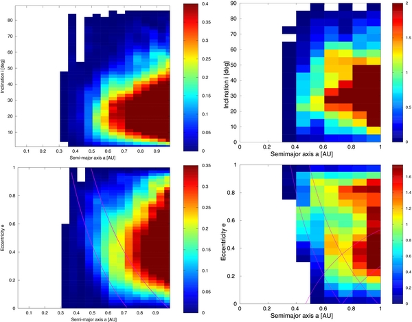
Figure 1. Residence time probability distributions from the Bottke et al. (2002) model (right) and the Greenstreet et al. (2012b) model (left). To monitor the orbital evolution of each particle, a grid of a, e, i cells was placed throughout the inner solar system from a < 4.2 AU, e < 1.0, and i < 90° with volume 0.1 AU × 0.05 × 500 for the Bottke et al. (2002) model and 0.05 AU × 0.02 × 200 for the Greenstreet et al. (2012b) model. These plots show only the a < 1.0 AU region. To create the a, e plot the i bins are summed and the e bins are summed to create the a, i plot. The color scheme represents the percentage of the steady-state NEO population contained in each bin. Red represents cells where there is a high probability of particles spending their time. The different stretch in color scales between the left and right panels is to compensate for the 5× larger cells in the Bottke et al. (2002) model. The curved lines indicate the crossing orbits of Earth, Venus, and Mercury.
Download figure:
Standard image High-resolution image3. TWO MODELS COMPARED TO NEOWISE ATEN DETECTIONS
To quantify the differences between the two model NEO orbital distributions, we have used the NEOWISE space telescope's detection biases published in Mainzer et al. (2012) to compare the orbital element distributions expected for the Aten population from the Greenstreet et al. (2012b) model as well as the Bottke et al. (2002) model with the detected NEOWISE Aten distributions. Figure 7 of Mainzer et al. (2012) provides the NEOWISE detection biases for the a, e, and sin(i) Aten distributions. We applied each bias to the a, e, and sin(i) Aten distributions from the Greenstreet et al. (2012b) model. Figure 2 shows the fractional distribution of the NEOWISE detections (blue), biased Bottke et al. (2002) model (black), and biased Greenstreet et al. (2012b) model (green) for the Aten a, e, and sin(i) distributions as histograms, and Figure 3 shows cumulative versions of the information. Although the Aten a, e, and sin(i) NEO distributions for both the biased Greenstreet et al. (2012b) and biased Bottke et al. (2002) models extend beyond the range shown in Figure 2, the NEOWISE Aten detections and thus the detection biases shown in Figure 7 of Mainzer et al. (2012) do not. Thus, to best compare the Greenstreet et al. (2012b) model, biased to the NEOWISE Aten detection biases, to the NEOWISE detections, we restrict the comparison to the same a, e, and sin(i) range in binning boundaries as used by Mainzer et al. (2012).

Figure 2. Fractional distribution of the a (top left), e (top right), and sin(i) (bottom left) NEOWISE detections (blue), biased Bottke et al. (2002) model (black), and biased Greenstreet et al. (2012b) model (green). There is little difference in a between the three distributions. In contrast, the e and sin(i) distributions expected from the Greenstreet et al. (2012b) model more closely match the NEOWISE detections than do the Bottke et al. (2002) expectations.
Download figure:
Standard image High-resolution image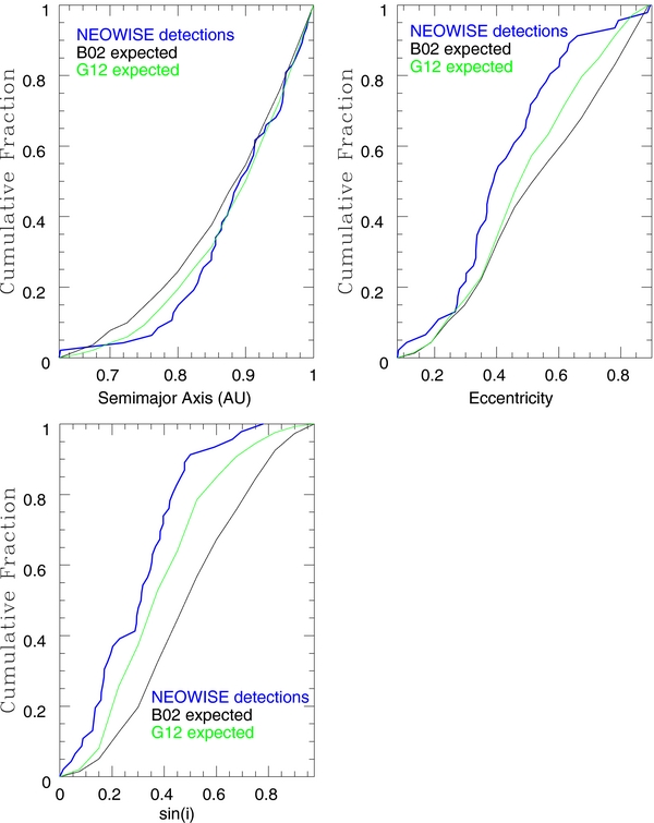
Figure 3. Cumulative distributions of the a (top left), e (top right), and sin(i) (bottom left) NEOWISE detections (blue), the biased Bottke et al. (2002) model (black), and the biased Greenstreet et al. (2012b) model (green). In all distributions, the Greenstreet et al. (2012b) model more closely matches the NEOWISE detections than do the expectations from the Bottke et al. (2002) model.
Download figure:
Standard image High-resolution image
3.1. Semimajor Axis Distributions
Examining first the semimajor axis distribution (top left of Figure 2), one can see only small variations between the expected distributions of the two models, with the main difference being that the Greenstreet et al. (2012b) model is shifted to a slightly larger fraction of Atens at high-a than the Bottke et al. (2002) model. These distributions are converted to the cumulative fraction less than a given a, e, or sin(i) value in Figure 3. The top left panel of Figure 3 shows the cumulative fraction less than a given semimajor axis for the NEOWISE detections (blue), the biased Bottke et al. (2002) model expectations (black), and the biased Greenstreet et al. (2012b) model expectations (green). One can see the Greenstreet et al. (2012b) model more closely matches the NEOWISE detections than the previous model, but the significance of this difference needs to be established. To quantify this comparison, a Kolmogorov–Smirnov (K-S) test was used to measure the probability of drawing the detected NEOWISE Aten semimajor axis distribution from the biased Bottke et al. (2002) model. The test gave a probability of 30% (Table 1), which is not rejectable at 99% confidence, the level we have chosen for near-certain rejection. The K-S test gives the probability of drawing the NEOWISE detections from the biased Greenstreet et al. (2012b) model as 80%, which is an acceptable match. Although a better match, this result alone would not lead us to strongly prefer the newer model.
Table 1. K-S Test Results
| a < 1 AU Orbital Model | a | e | sin(i) |
|---|---|---|---|
| (%) | (%) | (%) | |
| Bottke et al. (2002) | 30 | <0.5 | <0.01 |
| Greenstreet et al. (2012b) | 80 | 6 | 5 |
Note. Results of Kolmogorov–Smirnov tests for the probability of drawing each detected NEOWISE Aten distribution from the orbital element distributions of the Bottke et al. (2002) model and the Greenstreet et al. (2012b) model.
Download table as: ASCIITypeset image
3.2. Eccentricity and Inclination Distributions
The eccentricity distributions shown in the top right panel of Figure 2 show an overabundance of detected NEAs with moderate eccentricities at ∼0.3 to ∼0.4 and a relative deficit of high eccentricities (e > 0.674), compared to the predictions of the Bottke et al. (2002) model. A difference in the Aten eccentricity distributions for the two models is evident, with the Greenstreet et al. (2012b) model more closely following the detected distribution. The top right panel of Figure 3 gives a clearer picture of this difference, showing that the new model has a smaller fraction with e > 0.674. The K-S probability of drawing the NEOWISE Aten eccentricity detections from the Bottke et al. (2002) model is <0.5% (rejectable at >99% confidence), whereas the probability of drawing the NEOWISE detections from the Greenstreet et al. (2012b) model is 6% (an acceptable match).
Similarly, the inclination distributions shown in the final panel of Figure 2 clearly shows the relative deficit of detected high-i Atens that Mainzer et al. (2012) observed compared to the Bottke et al. (2002) model's expectations. This plot already makes it apparent that the Greenstreet et al. (2012b) model shares the lack of large orbital inclinations present in the NEOWISE detections. Once again, the K-S probability of drawing the NEOWISE Aten inclination distribution from the biased Bottke et al. (2002) model is rejectable at the >99% confidence level, whereas the biased Greenstreet et al. (2012b) model is not rejectable with a probability of 5%.
4. DISCUSSION
It is important to point out that for the a > 1.0 AU region, both the Greenstreet et al. (2012b) and Bottke et al. (2002) models agree with the NEOWISE detections. Figures 8 and 9 from Mainzer et al. (2012) show a comparison between the detected NEOWISE orbital element distributions and the Bottke et al. (2002) predictions for the Apollo (a > 1.0 AU, q < 1.017 AU) and Amor (1.017 < q < 1.3 AU) populations. This is perhaps unsurprising since the Amors and Apollos are the dominant NEA populations and are well characterized by the Spacewatch observations which were used to compile the Bottke et al. (2002) model. Although there are q ≪ 1.0 AU Apollos, the close encounter problems mentioned above, which must be present for the small fraction of objects, are fractionally less and do not cause a detectable problem. The main difference between the two models is thus in the low-a region as has been shown in this Letter.
For this preliminary study we chose a 99% confidence level before confidently rejecting a model expectation. However, our e and sin(i) distributions are approaching being rejectable at a 95% confidence level. We believe that some part of the remaining discrepancy is that we have used one-dimensional biases computed for the wrong orbital distribution. That is, Mainzer et al. (2012) computed the inclination bias (for example) for the a/e distribution of the Bottke et al. (2002) model, and thus our use of the given sin(i) bias is not rigorously correct. However, although differences in the two orbital distributions are apparent, their gross features are generally similar. As can be seen in Figure 1, the general trend in both a/e distributions for the a < 1.0 AU region is a monotonic decrease in the a population from a near 1 AU to smaller semimajor axes and a peak in the e distribution near ∼0.4 with a smaller fraction of the population at lower and higher eccentricities. The a/i distributions for both models have a peak between i ∼ 20° and i ∼ 30° with less of the population at lower and higher inclinations. We believe the recomputed biases using the Greenstreet et al. (2012b) model would not be hugely different from the current biases that use the Bottke et al. (2002) model due to these general similarities between the two orbital models. Recomputing the biases is a major computational effort (A. Mainzer 2012, private communication). It is unclear how the complex pointing history of the NEOWISE spacecraft transforms the three-dimensional orbital element distribution into the three one-dimensional biases, making it difficult to estimate how different the "corrected" biases would be. Nevertheless, to improve the analysis presented in this Letter, the NEOWISE detection biases should be recomputed using the Greenstreet et al. (2012b) model and will be the subject of future work. It is plausible this will further improve the match of the Greenstreet et al. (2012b) model to the NEOWISE detections.
If a mismatch between the model and the detections had been found, one may have been inclined to invoke non-gravitational physics into the model. The effects which can cause NEAs to migrate in semimajor axis could include radiation pressure (Vokrouhlický & Milani 2000) and the Yarkovsky effect (Farinella & Vokrouhlický 1999; Bottke et al. 2000); once km-scale NEAs are strongly coupled to the planets these slow effects may become negligible in the long-term orbital evolution. Nevertheless, one could imagine that tidal disruption by planetary encounters (Richardson et al. 1998) or perhaps more frequent collisions in the reduced volume closer to the Sun (Grun et al. 1985) could change the relative orbital distribution of low-a objects. Given the acceptable match between the Greenstreet et al. (2012b) NEO orbital model and the detected NEOWISE Aten orbital element distributions, in particular the rarity of large-inclination Atens, a purely gravitational model is non-rejectable, and thus no additional physics is required.
S. Greenstreet and B. Gladman acknowledge support from NSERC and CSA. We acknowledge CSC–IT Center for Science Ltd. for the allocation of computational resources. This research has been enabled by the use of Compute/Calcul Canada computing resources provided by WestGrid and the SciNet HPC Consortium.