


ABSTRACT
Mass escape rate of mon- and diatomic gases from a planetary atmosphere is studied based on Parker's model for a broad range of surface conditions. The escape rate is found to follow two asymptotic regimes, namely, high- and low-density regimes, with a short intermediate regime between them. Equations for the escape rate in every asymptotic regime are found theoretically. A comparison of the obtained escape rates with results of recent kinetic simulations shows that Parker's model satisfactorily predicts escape rates only in the high-density regime. Based on this finding, a criterion of applicability of Parker's model for the calculation of the mass escape rate is established.
Export citation and abstract BibTeX RIS
1. INTRODUCTION
Hydrodynamic modeling based on equations of continuum fluid flows is one of the major approaches for simulation of thermally escaping atmospheric flows. Historically, such models were first applied to study a similar phenomenon of solar wind flow. In particular, Parker (1964a, 1964b) developed a one-dimensional hydrodynamic model of thermal escape from solar corona, assuming that the temperature drops to zero far from the star. Later on, Parker's model became a basis for numerous studies of thermal escape from atmospheres of planetary bodies in the outer solar system (e.g., Watson et al. 1981; Chassefière 1996; Krasnopolsky 1999; Strobel 2008; Zhu et al. 2014) and exoplanets (e.g., Tian et al. 2005; Muñoz 2007).
In order to satisfy the condition of zero temperature far from the surface, it is necessary to continue solution of Parker's model above the exobase into exosphere, where the Fourier law for the heat flux fails (e.g., Volkov et al. 2011a). In spite of this basic flaw, Parker's model has never been systematically tested against kinetic models, which can accurately predict the heat flux and structure of non-equilibriums flow in the exosphere. Thus, the usefulness of Parker's model for thermal escape problems remains questionable.
One-dimensional steady-state hydrodynamic equations of inviscid thermally conducting gas flows have a few distinct types of solutions depending on conditions far from the surface (Freeman & Johnson 1972; Roberts & Soward 1972), including the Chamberlain-type solar breeze solutions with decreasing velocity in the far field (Chamberlain 1961, 1965) and Parker-type solutions with monotonously increasing gas velocity (Parker 1964a, 1964b). The kinetic simulations predict the solar-breeze-type thermally escaping solutions only in conditions of the atmospheric blow-off or transition from the blow-off to Jeans-like escape (Volkov 2014). In the present letter, thermal escape in the Jean-like regime is considered, when the kinetic simulations (Volkov et al. 2013) predict monotonously increasing gas velocity, so that only Parker-type hydrodynamic solutions are chosen for comparison.
The present letter reports for the first time results of systematic comparison of thermal escape rates obtained in hydrodynamic and kinetic simulations. Based on this comparison, the range of surface conditions is found, where Parker's model can be used for calculations of the escape rates. It is shown that Parker's model satisfactorily predicts the escape rate only in the so-called high-density (HD) asymptotic regime. The criterion, determining surface conditions for which Parker's model is capable of quantitative prediction of the escape rate is then established theoretically. Although both hydrodynamic and kinetic simulations are performed for atmospheres without heating, the obtained criterion can be also used to assess the applicability of Parker's model in the externally heated atmospheres based on the parameters on the top of heated atmospheric layer as it is discussed in Section 6.
2. PARKER'S MODEL OF THERMAL ESCAPE
In one-dimensional steady-state atmospheric flows without heating, the distributions of gas density ρ, velocity u, and temperature T can be described by the Navier–Stokes equations


where r is the radial distance, the prime symbol denotes derivatives with respect to r, 
 kB is the Boltzmann constant, m and ζ are the mass and number of internal degrees of freedom of a molecule, M is planet's mass, G is the gravitational constant, Φm and Φe are the mass and energy escape rates per steradian, and τrr and qr are the viscous stress and heat flux. Atmospheric flows are usually sought with constrains on the surface density ρ0 and temperature T0:

where r0 is the surface radius, and the density is assumed to drop to zero far from the planet:

Two more boundary conditions are necessary to solve Equations (1), since Φm and Φe are unknown.
Parker (1964a, 1964b) made three basic assumptions, which helped him to resolve the issue of the missing boundary conditions. First, he considered outflows with a monotonically increasing velocity, which is much smaller than the isothermal sound velocity  at the surface. Second, he assumed that the molecular viscosity plays a marginal role, in which case Equations (1) can be reduced by neglecting τrr, so that


where the Fourier law,  with thermal conductivity,
  is assumed for the heat flux, and ω is the viscosity exponent. Equations (4) require four boundary conditions, so that Parker (1964a, 1964b) finally assumed that the temperature should drop to zero far from the surface:

In this model, the isothermal Mach number  evolves from
  at r = r0 to infinity at
  i.e., the flow passes through the isothermal sonic point, where
  and the denominator of Equation (4a) is equal to zero. Distributions of gas parameters are continuous only if the numerator becomes zero simultaneously with the denominator, i.e., the isothermal sonic point is the critical point of Equations (4). Using Equation (4b) in order to exclude T' from the consideration at the critical point, one can obtain

where subscript "c" denotes parameters in the critical point. This equation shows that gas parameters at the critical point and escape rates are not independent of each other. For a solution passing through the critical point with monotonically increasing velocity, the density drops as 1/r2 far from the surface and Equation (3) is satisfied automatically, so it should be excluded from consideration and replaced by Equation (6).
Thus, Parker's model implies a solution of Equation (4) with boundary conditions given by Equations (2) and (5) starting at the surface with  and passing through a critical point, where atmospheric parameters satisfy Equation (6).
3. NUMERICAL APPROACH FOR SOLVING EQUATIONS OF PARKER'S MODEL
In the present paper, Parker's model is analyzed in a dimensionless form in order to reduce the number of parameters governing the solutions. Equation (4) is re-written in terms of dimensionless variables 
 and
and  as
as


where the prime symbol denotes derivatives with respect to 
 is the Jeans parameter at the critical point,
  and
and  Equation (6) in reduced units transforms into

Solution of Parker's model in reduced units depends only on two surface parameters, e.g., Jeans parameter  and Knudsen number
  characterizing the strength of the gravitational field and degree of atmosphere rarefaction at the surface. Assuming that the mean free path of gas molecules
  is given by the first approximation of the Chapmen-Enskog theory for the Variable Hard Sphere (VHS) molecular model (Bird 1994), and the atmospheric length scale L0 is equal to r0, one can find that
  =
=  , where
  is the Knudsen number at the critical point

and Pr is the Prandtl number.
A solution of Equation (7) for the surface conditions given by λ0 and Kn0 can be obtained using a two-step approach. At the first downstream step, Equation (7) is solved in the downstream direction from the critical point,  for a fixed λc with the initial conditions

and Ψe given by Equation (8). These equations are solved iteratively by varying  until a
  is found that the condition

is satisfied. By repeating this iterative procedure for various λc, the dependence  can be obtained numerically. At the second upstream step, Equation (7) are solved with the initial conditions given by Equation (10) in the upstream direction,
  for fixed λ0 and Kn0. For Kn0 < Knc, one can iteratively find such λc and
  that Jeans parameter and Knudsen number at
  are equal to λ0 and Kn0. Once the dependences
  and
and  are established, they can be used in order to find any solution of Parker's model for a given surface condition. Typical dependences of λc on λ0 and Kn0 are shown in Figure 1. It is remarkable that λc varies within a narrow range at small Kn0 and large λ0 for arbitrary γ and ω.
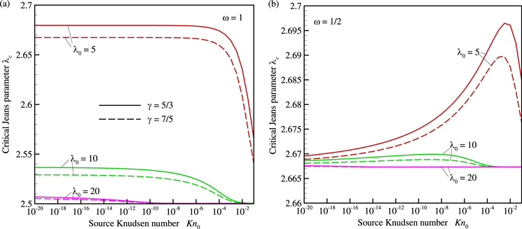
Figure 1. Jeans parameter at the critical point λc vs. surface Knudsen number Kn0 obtained with Parker's model at γ = 5/3 (solid curves) and γ = 7/5 (dashed curves) for ω = 1 (a) and ω = 1/2 (b) and various surface Jeans parameters: λ0 = 5, λ0 = 10, and λ0 = 20.
Download figure:
Standard image High-resolution image4. ESCAPE RATES IN PARKER'S AND KINETIC MODELS
Numerical calculations with Parker's model were performed for mon- ( γ = 5/3) and diatomic (ζ = 2, γ = 7/5) gases with Pr = 2/3 and for ω = 3/4, and ω = 1. The mass escape rate is calculated in reduced units as

where Ma0 and  are the Mach number and Jeans escape rate at the surface:


The dependences of  on Kn0 at fixed λ0 are found to be qualitatively similar for all γ and ω considered and include two asymptotic regimes, which correspond to the case of large and small Kn0, and intermediate regime, corresponding to transition between these asymptotic regimes (Figure 2(a)). Following Parker (1964b), the case, when
  asymptotically does not depend on Kn0, can be called the low-density (LD) regime and the case, when
  asymptotically varies as 1/Kn0, can be called the HD regime.
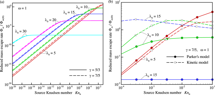
Figure 2. Reduced mass escape rate  vs. surface Knudsen number Kn0 for various λ0. In panel (a), all curves are obtained with Parker's model for γ = 5/3 (solid curves) γ = 7/5 (dashed curves) at ω = 1. In panel (b), curves are obtained for γ = 7/5 and ω = 1 with the kinetic (Volkov et al. 2011a, 2013; dashed curves) and Parker's (solid curves) models.
Download figure:
Standard image High-resolution imageThe escape rates calculated with Parker's model are found to be in quantitative agreement with results of recent kinetic simulations performed by Volkov et al. (2011a, 2013) only in the HD regime (Figure 2(b)), when values of  calculated with both models asymptotically approach each other with decreasing Kn0 as it is seen for λ0 = 5 and λ0 = 10. At λ0 = 15, the escape rates disagree in the considered range of Kn0, but they presumably agree at smaller Kn0, where the results of kinetic simulations are not currently available. In the LD regime, kinetic
  approaches
  at
at  when the effects of intermolecular collisions become progressively less important and escaping flows evolve in the free molecular flow regime. On the contrary,
  predicted by Parker's model at
  can be both larger and many orders of magnitude smaller than 1. For instance, in the range
  = 15–20, which is characteristic for a number of large Kuiper Belt objects (KBOs, Johnson et al. 2015), the maximum values of
  are in the order of 10−2–10−4.
5. CRITERION OF VALIDITY OF PARKER'S MODEL
The goal of the present section is to formulate a criterion of validity of Parker's model in terms of λ0 and Kn0 for arbitrary γ and ω. For this purpose, accurate expressions for  in both HD and LD regimes are obtained first.
In the LD regime, the Knudsen number is large everywhere, including at the critical point, and  is small according to Equation (9). Following Parker (1964b), one can consider the only case when
  and integrate Equation (7b) neglecting all terms in the right-hand side of this equation with exception of Ψe. Solution of the obtained equation satisfies Equation (11) if
 and temperature varies as (Parker 1964b)

The critical Jeans parameter in the LD regime  corresponds to the minimum possible λc for a gas with given ω. If
  then the term with
  in the right-hand side of Equation (7a) can be neglected and gas velocity far upstream of the critical point varies as (A. N. Volkov 2015, in preparation)

where the coefficient  is given by the condition that Equation (16) matches the accurate solution of Equation (7a) at
  The analysis of numerical solutions of Parkers model showed that V0(ω ) varies from ∼0.708 to ∼0.6725 when ω increases from 1/2 to 1 and can be fitted to the power law
  Since
Since 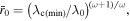 Equations (15) and (16) allow one to calculate the surface Mach number
  and escape rate
  in the LD regime as


In order to find an equation for the escape rate in the HD regime the definition of λ0 can be re-written to represent the surface temperature as a function of λ0 and Kn0:

With exception of the case, when λ0 is close to  solutions of Parker's model at various λ0 correspond to
  (Figure 1). Such "upstream" solutions start at large Knudsen numbers at the critical point and then, with decreasing
  first follow Parker's LD approximation. Then they gradually approach another limit solution corresponding to the case of small surface Knudsen number, i.e., Parker's HD approximation. Then surface temperature and its gradient can be found as


Equation (7b) can be re-written at  as
as

By excluding the derivative from Equations (21) and (22) in the HD regime, when  and
and  one can obtain

This equation can be used in order to calculate the surface Mach number and escape rate in the HD regime based on Equation (12) as


The numerical values of the escape rate closely approach the solutions given by Equations (18) and (25) as shown in Figure 3 for γ = 7/5 and ω = 1. Calculations for γ = 5/3 and/or various ω from 1/2 to 1 demonstrate similar degree of agreement between obtained equations and numerical  Both equations, however, become inaccurate when λ0 closely approaches

Figure 3. Reduced mass escape rate  vs. Knudsen number Kn0 obtained as a result of direct numerical solution of Equation (7) (dashed–dotted curves), with Equation (18) for the HD regime (dashed lines), and with Equation (18) for the LD regime (solid curves) at γ = 7/5, ω = 1, and λ0 = 5, λ0 = 10, and λ0 = 20. Dashed-double-dotted line corresponds to points where
  or Kn0 = KnP.
Download figure:
Standard image High-resolution imageAs it was shown in Section 4, Parker's model enables quantitative prediction of Φm only in the HD regime. Based on Equations (17) and (24), this criterion of validity of Parker's model can be now formulated as

or

where the "turning" Knudsen number KnP

corresponds to the nominal point where the dependence of the escape rate Kn0 turns from the LD to HD regime. A comparison of Parker's solutions with results of kinetic simulations at λ0 = 5 and λ0 = 10 shows that Parker's escape rate is within a factor of two from the kinetic rate if  The turning Knudsen number, KnP, is a strong function of ω, but only marginally depends on γ (Figure 4). At fixed λ0, Parker's model is valid in a substantially broader range of Kn0 in the pseudo-Maxwellian gas (ω = 1) than in the hard sphere gas (ω = 1/2).

Figure 4. Turning Knudsen number KnP given by Equation (28) vs. surface Jeans parameter λ0 for γ = 5/3 (solid curves) and γ = 7/5 (dashed curves) at ω = 1/2, ω = 3/4, and ω = 1.
Download figure:
Standard image High-resolution imageThe criterion of validity of Parker's model can be also formulated in terms of integral atmospheric parameters, which can be directly deduced from the analysis of absorption spectra of planetary bodies or probing the atmospheres during stellar occultation, e.g., the column density N

Here rx is the radial position of the nominal exobase, where the mean free path of gas molecules  is equal to the atmospheric scale height
  (
( is the exobase Jeans parameter). Assuming the barometric distribution of molecules with the scale height
 the first approximation to the column density at large λ0 is

where for the VHS model of intermolecular collisions ![${{\rm{\Sigma }}}_{T}\left({T}_{0}\right)={k}_{{\rm{B}}}\sqrt{{\mathfrak{R}}{T}_{0}}/[K\kappa ({T}_{0})]=\sqrt{2}{\sigma }_{T}({T}_{0})$](https://content.cld.iop.org/journals/2041-8205/812/1/L1/revision1/apjl520423ieqn78.gif) and
and  is the total collision cross section of molecules at temperature T0 (Johnson et al. 2015) with typical value in the order of 10−14 cm−2 for atmospheric species like N2 or CH4 (Bird 1994). The examples of dependences of N/N0 on Kn0 at various λ0 obtained for a monatomic gas with ω = 1 are shown in the inset of Figure 5. It is seen that N/N0 is independent of Kn0 if Kn0 < 10−5. Calculated values of N/N0 in the limit of small Kn0 are shown in Figure 5 by symbols. These values marginally depend on γ and ω, so that the ratio N/N0 can be considered as a function of only λ0 and fitted at λ0 ≥ 4 by equation

shown in Figure 5 by the solid curve. Then the criterion given by Equations (27) and (28) can be reformulated in terms of N as


Figure 5. Reduced column density N/N0 vs. Jeans parameter λ0 obtained with Parker's model in the limit  at ω = 1/2 (square symbols) and ω = 1 (triangle symbols). Solid curve corresponds to Equation (31). Calculated values of N/N0 for γ = 5/3 and γ = 7/5 visually coincide with each other at
  The inset shows N/N0 vs. Kn0 obtained at γ = 5/3 and ω = 1 for λ0 = 5, λ0 = 10, and λ0 = 20.
Download figure:
Standard image High-resolution image
6. DISCUSSION AND CONCLUSION
The developed criterion for the validity of Parker's model for thermal escape problems can be directly applied for atmospheres without substantial external heating. Certain KBOs, including dwarf planets in the outer solar system, may have such atmospheres. The degree of absorption of solar radiation in KBO atmospheres depends on atmospheric column (Johnson et al. 2015) and, in particular, on the abundance of methane, which is the primary absorbing agent in presumably nitrogen-rich KBO atmospheres (Strobel et al. 1996; Krasnopolsky & Cruikshank 1999). Currently the abundance of methane is not well-constrained for the majority of KBOs with exception of Pluto and Charon (see review of literature data, e.g., in Johnson et al. 2015). For Sedna and Quaoar, which have relatively thin and thick atmospheres (N ≈ 1017 cm−2 and N ≈ 1021 cm−2) at λ ≈ 15 in solar-maximum conditions (Johnson et al. 2015), Kn0 ≈ 7 · 10−5 and Kn0 ≈ 7 · 10−9, while Knp ≈ 5 · 10−8. For KBOs like Pluto with larger λ0, the condition given by Equation (28) is even more restrictive. Thus, Parker's model is not applicable for the majority of KBOs, which atmospheres do not contain sufficient amount of CH4 to be heated by solar radiation.
For planetary atmospheres with external heating, the criterion given by Equation (28) can be used with certain approximations, assuming that λ0 and Kn0 characterize flow conditions at the top of the heated layer. These conditions are more favorable for application of Parker's model above the heated layer because of increase in the local Jeans parameter. With increasing amount of absorbed energy and decreasing Jeans parameter at the upper boundary of the heated layer, the critical point approaches the exobase, and Parker's and kinetic model can produce similar escape rates as it is apparent from the comparison of curves for λ0 = 5 in Figure 2(b). This is in agreement with findings by Zhu et al. (2014), who concluded that Pluto's exobase is locked at λx = 4–6, and Parker's model escape rate is different from the enhanced Jeans rate predicted in kinetic simulations by Volkov et al. (2011a, 2011b) by the factor of 1–0.22. For less intensive heating, which can be specific to other dwarf planets, Parker's model applied to the part of the atmosphere above the heated layer can substantially underestimate the escape rate.
In conclusion, the numerical study of Parker's model reveals that two asymptotic regimes can occur depending on the surface conditions. The escape rates in these regimes are calculated theoretically in the form of Equations (18) and (25). Escape rates predicted by Parker's and kinetic models agree only in the HD asymptotic regime. The criterion of applicability of Parker's model is then given by Equations (27) and (28) or (32).
This research was supported by the NASA Planetary Atmospheres Program. The author thanks Prof. R. E. Johnson for helpful comments on the results discussed in the present paper.