


ABSTRACT
We present a model for the narrow, ribbon-like enhancement in the emission of ∼keV energetic neutral atoms (ENA) coming from the outer heliosphere, coinciding roughly with the plane of the very local interstellar magnetic field (LISMF). We show that the pre-existing turbulent LISMF has sufficient amplitude in magnitude fluctuations to efficiently trap ions with initial pitch-angles near 90°, primarily by magnetic mirroring, leading to a narrow region of enhanced pickup-proton intensity. The pickup protons interact with cold interstellar hydrogen to produce ENAs seen at 1 AU. The computed width of the resulting ribbon of emission is consistent with observations. We also present results from a numerical model that are also generally consistent with the observations. Our interpretation relies only on the pre-existing turbulent interstellar magnetic field to trap the pickup protons. This leads to a broader local pitch-angle distribution compared to that of a ring. Our numerical model also predicts that the ribbon is double-peaked with a central depression. This is a further consequence of the (primarily) magnetic mirroring of pickup ions with pitch-angles close to 90° in the pre-existing, turbulent interstellar magnetic field.
Export citation and abstract BibTeX RIS
1. INTRODUCTION
A narrow band of energetic neutral atoms (ENA) originating in the outer heliosphere, known as the "IBEX ribbon," was discovered by the Interstellar Boundary Explorer spacecraft (Funsten et al. 2009; Fuselier et al. 2009; McComas et al. 2009; Möbius et al. 2009; Schwadron et al. 2009). Numerous models of its origin have been proposed (cf. McComas et al. 2014). A similar ENA emission was discovered by Cassini/INCA (Krimigis et al. 2009). It is widely believed that the ribbon nearly coincides with the direction normal to the local interstellar magnetic field (LISMF; Schwadron et al. 2009). A popular model for explaining this was suggested by McComas et al. (2009) and worked out quantitatively by Heerikhuisen et al. (2010). In this model, the emission is the result of the interaction of ∼keV-energy pickup protons beyond the heliopause with cold interstellar neutral H. A requirement of the model is that the pickup protons gyrate normal to the LISMF for a year or more. Florinski et al. (2010) noted that the such a distribution would excite magnetic fluctuations on a much shorter timescale, causing the protons to become isotropic, and there should be no ribbon (see also Gamayunov et al. 2010). Schwadron & McComas (2013) proposed a solution to this puzzle in which enhanced magnetic fluctuations trap the pickup protons, forming a spatial structure, or region, of increased particle density beyond the heliopause, which is the source of the ribbon (see also Isenberg 2014).
Recently, Burlaga et al. (2015) reported Voyager 1 (V1) observations of the small-scale end of the interstellar magnetic field turbulence spectrum (Burlaga et al. 2015). These observations are consistent with those of interstellar density and magnetic field turbulence over a wide range of scales (e.g., Minter & Spangler 1996). There is no evidence for an enhancement due to pickup-ion generated waves.
Here we give a new interpretation for the IBEX ribbon that relies on the trapping of protons by the pre-existing turbulent fluctuations in the LISMF magnitude, primarily through the effect of magnetic mirroring. Magnetic mirroring of particles in the compressed LISMF near the heliopause was previously discussed by others (McComas et al. 2009; Schwadron et al. 2009; Chalov et al. 2010), but its importance as a means for trapping pickup ions within pre-existing turbulence has not previously been recognized. We start with a simple theory that predicts the width of the ribbon and then present a detailed numerical model that also gives its absolute flux.
2. ANALYTIC MODEL
Consider the illustration in Figure 1. Fast neutral particles (solid arrows ) are produced by the charge exchange between solar wind protons moving with speed Vw, and nearly stationary interstellar neutral atoms, and then move radially outward from the Sun until they are ionized by charge exchange with thermal protons in the local interstellar plasma. Upon ionization in the interstellar plasma, the resulting pickup-proton moves in the LISMF with a speed Vw. These are so-called "secondary pickup protons" and are indicated with wavy curves, representing their gyromotion, in Figure 1. After some time, these again undergo charge exchange with cold interstellar atoms, leading to other fast neutral atoms (these ENAs are not shown in the figure). Some of these ENAs return to 1 AU where they are observed.

Figure 1. Cartoon illustration of our model. The gray shaded regions indicate places where the initial pitch-angle of secondary protons are small enough to be magnetically mirrored by small-amplitude fluctuations in the turbulent LISMF, enhancing the pickup-proton intensity there.
Download figure:
Standard image High-resolution imageInitially, a secondary proton has a pitch-angle cosine, μ0, relative to the local magnetic field vector,  , given by μ0 = Br/B, where Br is the radial component of the LISMF in a Sun-centered coordinate system, and
The LISMF consists of a mean and a fluctuating component arising from interstellar turbulence. The ∼1018 cm outer scale of interstellar density turbulence is extremely large compared to the pickup-proton gyroradius. Thus, the magnetic moment of the secondary protons, W⊥/B, where W⊥ is the kinetic energy in components of the proton velocity vector normal to  , is approximately constant. The turbulence on scales smaller than the gyroradii of the particles have very small amplitudes. From quasi-linear theory, one finds the mean-free path for scattering of 1 keV protons in the turbulent interstellar magnetic field to be some 10 times larger than the size of the heliosphere.1
The ribbon-producing particles have very small pitch cosines and quasi-linear theory is known to breakdown in this regime. Magnetic mirroring likely plays an important role (see Jones et al. 1978).
, is approximately constant. The turbulence on scales smaller than the gyroradii of the particles have very small amplitudes. From quasi-linear theory, one finds the mean-free path for scattering of 1 keV protons in the turbulent interstellar magnetic field to be some 10 times larger than the size of the heliosphere.1
The ribbon-producing particles have very small pitch cosines and quasi-linear theory is known to breakdown in this regime. Magnetic mirroring likely plays an important role (see Jones et al. 1978).
The timescale for the variation in  at the relevant ∼10–100 AU scales, and a wave speed of ∼50 km s−1, is about a year, so we may consider a static magnetic field. In this case, the proton kinetic energy is constant, so that the conservation of magnetic moment implies
  = constant. Because of turbulent variations in B, μ also varies. μ will decrease for protons that move toward increasing B until B is sufficiently strong to mirror it backward. Particles with μ ≈ 0 can be mirrored by rather small increases in B, leading them to effectively be trapped. By equating the magnetic moment at the start of the secondary proton trajectory to that at its mirror point, at which point μ = 0, we find a criterion for which particles can be quasi-trapped:

where  is the value of the field at the mirror point. We have assumed that the particle starts with a finite μ which then decreases as B becomes stronger (δB > 0).
The gray shaded region in Figure 1 is where particles have sufficiently small μ0 that they satisfy Equation (1) and are quasi-trapped. The angle φ is related to μ0. Note that  where α is the pitch-angle. Thus,
  In our model, the trapping is due to pre-existing fluctuations only, rather than due to self-excited waves (Schwadron & McComas 2013).
δB in Equation (1) is the rms amplitude of the pre-existing turbulent magnetic field magnitude fluctuations. We consider a Kolmogorov spectrum of turbulence of the form  where Lc is the outer scale, k is the wavenumber, and
  is the global variance. We are interested in fluctuations with spatial scales, lH, the size of the heliosphere, because secondary protons do not move far enough to sample the entire range of scales of turbulent interstellar fluctuations during their 1–2 year lifetime. Thus,

where kH = 2π/lH. We have assumed the same form for P(k) as Giacalone & Jokipii (1999; see their Appendix B, Equation (B3) et seq.), which is also that used in the numerical model discussed in the next section. The angle φ, as discussed above, is given by  Thus, we have:

where we have assumed  where BISM is the average interstellar magnetic field strength.
To estimate lH, we note that the density of secondary protons outward from the heliopause, r = Rhp, falls off roughly exponentially because of losses due to charge exchange with cold interstellar H. The characteristic scale, λi, is of the order of 100 AU. Thus, we take  Inserting this into Equation (3), solving for φ, and taking γ = 5/3, we find

Taking Lc = 4 pc,  BISM = 3 μG, and B0 = 4.6 μG (Burlaga & Ness 2014), we find φ = 0.21 rad., which is about 12°. This of the same order as the observed thickness of the ribbon reported by Fuselier et al. (2009) and Schwadron et al. (2014). We have neglected the bending (or "draping") of the interstellar magnetic field lines near the heliopause, which may also contribute to the observed width (e.g., Isenberg et al. 2015; Zirnstein et al. 2015).
Because of the fluctuations in  , the distribution of secondary protons is broadened about μ0. In Equation (1), we considered the case in which μ decreased (from μ0) while B increased as the particle moved toward the mirror point. Since B is a random function, it will have both increases and decreases. Thus, we expect particles within the gray shaded region of Figure 1 to have a range of μ values and the distribution to peak near 0 with a width of the same order as the ribbon. Florinski et al. (2010) found that a perfect ring-beam distribution (μ = 0) is unstable and will lead to the growth of fluctuations in
  . We suggest the local distribution will be considerably broader than a pure ring-beam distribution leading to a longer timescale for wave growth than that estimated by Florinski et al. (2010).
3. NUMERICAL MODEL AND RESULTS
To more accurately model the propagation of protons in the turbulent LISMF we numerically integrate their equations of motion in a pre-defined magnetic field. The protons have a constant speed Vw. In this model, we assume that fast neutral atoms move without ionization inside the heliosphere, whose boundary is assumed to be Rb (=100 AU). This is essentially the heliopause in our calculation and is shorter than the actual location of the heliopause ∼20 AU further out (Gurnett et al. 2013), but the value of Rb does not significantly affect our primary conclusions, so we have chosen it to be 100 AU. The initial location of each secondary proton is determined from a spherically symmetric distribution, centered at the Sun, at a heliocentric distance determined from an exponential probability distribution with a characteristic scale, λi, of 100 AU, beyond Rb (all particles have r > Rb). Proton trajectories are followed until they are re-neutralized in a time determined from an exponential distribution with a characteristic time, τi = λi/Vw, which is just over a year.
The LISMF is determined kinematically by superimposing a random fluctuating component onto a mean. The field is assumed to be static, as discussed above. The global mean magnetic field is arbitrarily taken to be  where the x − y plane is the same as the solar equatorial plane and z points north. We consider a single realization of the random field. The local mean magnetic field in the vicinity of the heliosphere for this realization is different from the global mean and lies mostly in the y − z plane, having coordinates of approximately
  We neglect the draping of the magnetic field around the heliopause. The turbulent field is generated by summing over a large number of randomly directed plane waves (Giacalone & Jokipii 1999). The amplitude of each is determined from an assumed power spectrum, P(k), as discussed before. The longest wavelength is 20 pc, the shortest is 0.5Vw/Ωp (where Ωp is the proton gyrofrequency), and Lc = 4 pc. The logarithmic spacing between wave numbers is dk/k = 0.05. The total integrated variance, over all scales, is set equal to
  We also assume isotropic turbulence, for convenience, which gives rise to significant fluctuations in the magnitude of the magnetic field when the variance is of the order of the mean, as we consider here. The dashed lines in Figure 1 are magnetic field lines determined from our model magnetic field. While the field lines appear to vary only slightly, these small variations significantly affect the particle motion.
The equations of motion of approximately 4 million secondary protons were integrated numerically using the same method as Giacalone & Jokipii (1999). Because there is no electric field, the proton kinetic energy remains constant throughout the numerical integration.
Because our model LISMF does not depend on time, the distribution function, f, of secondary protons can be determined by binning along each particle's trajectory, provided the binning is at equal time intervals (see Giacalone 2005). f depends on three heliocentric spatial coordinates (r, θ, ϕ) and the particles' pitch cosine relative to the local magnetic field, μ. We use 50 logarithmically space bins in r such that Rb < r < 20Rb (100–2000 AU). There are 50 equally spaced values of 0 < ϕ < 360° and  respectively, and 200 equally spaced values of −1 < μ < 1. f is assumed to be independent of the particle gyrophase (which is computed along the trajectory). A typical proton is followed for about
  and f is binned every
f is normalized such that the total number of particles is equal to the flux of fast neutral atoms from the heliosphere crossing Rb multiplied by the surface area of the sphere,  multiplied by the average lifetime of the secondary protons, τi. Thus,
  where nfn is the number density of fast neutrals at r = Rb. We take this to be the same as the number of pickup ions (ionized interstellar atoms within the heliosphere) at this location and take
  corresponding to a pickup-ion density of ∼20% of that of the solar wind density at 100 AU (see Giacalone & Decker 2010). In the integral above,
  where p is the particle momentum and dE = 0.5 keV (see Florinski et al. 2010; Heerikhuisen et al. 2010).
The differential intensity, JENA, of ENAs produced after the secondary protons have re-neutralized, observed at 1 AU is  where Jsp is the differential intensity of secondary protons (=fp2). The factor 1/λi is a combination of the cross-section for ionization and neutral H density. μ' is the value of μ for which the velocity vector points opposite of the line of sight, which is taken to be the radial direction. Since μ is measured relative to the local magnetic field, the calculation of JENA involves the local magnetic field, which is known at each location.
Figure 2 (a) shows JENA in a standard Mollweide projection of latitude and longitude. The central meridian corresponds to ϕ = 0 and the equator is where θ = π/2. The black curve is where the model LISMF at r = Rb is normal to the radial direction. The concentration of ENAs that are roughly coincident with this curve is consistent with observations and the general physical picture of Heerikhuisen et al. (2010). The absolute flux in our model, for this particular choice of parameters, is of the same order as that observed. The thick white dashed lines are cross-sections of the ENA emission shown in Figure 2(b), and the solid white circles are the locations of the pitch-angle distributions shown in Figure 3(a).
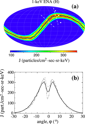
Figure 2. (a) Global map of the 1-keV energetic neutral hydrogen differential intensity, J, in a classic Mollweide projection. White dashed curves represent equal intervals in longitude (30°) and latitude (15°). The central meridian is a longitude of 0, and the equator is a latitude of 0. The black curve is the projection of the plane of the LISMF (this is where  ). (b) Cross-sections of J normal to the black curve shown in (a) as a function of the angle relative to the center of the ENA emission (black curve). The thick solid curve is the average over many cross-sections. The thinner dashed (dotted–dashed) curve corresponds to the cross-section centered at the longitude/latitude: 58°/38° (14°/20°), respectively. These cross-sections are shown as white dashed lines in panel (a). The solid circles are the locations of the pitch-angle distributions shown in Figure 3.
Download figure:
Standard image High-resolution image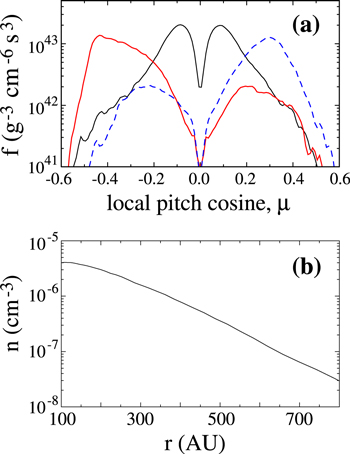
Figure 3. (a) Distribution function of secondary protons as a function of the pitch cosine relative to the local magnetic field at r = 110 AU for three separate longitude/latitude coordinates in the Mollweide projection shown in Figure 2: the 75°/37 5 black curve (center of the ribbon), the 75°/15° red curve (below the ribbon), the 75°/60° blue dashed curve (above the ribbon). These locations are shown as solid white circles in the top panel of Figure 2. (b) The density of secondary protons as a function of radial distance for protons, averaged over all longitudes and latitudes along the black curve shown in Figure 2.
Download figure:
Standard image High-resolution image
The width of the modeled ribbon can be estimated by inspection of Figure 2(b). The abscissa is the angle of a spatial cross section of JENA, normal to the ribbon. The thick black curve is averaged over many spatial cross-sections, and the thinner dashed and dotted–dashed curves are two individual cross-sections. The full width at half maximum is about 25°, which is consistent with that observed (Fuselier et al. 2009; Schwadron et al. 2014), and estimated theoretically in the previous section. As noted above, the draping of the interstellar magnetic field around the heliopause may also contribute to the observed width, but this is neglected in our model.
Our model also predicts that the flux of ENAs as a function of the angle φ has two peaks, with a depression near the curve where  This double-humped ENA feature (which is related to the local pitch-angle distribution discussed further below) is seen in both the individual and average cross-sections. In the longitude-latitude map shown in Figure 2(a), it appears as a double-banded structure. To our knowledge, this feature has not been previously reported. There is a 5°–10° separation between the peaks, which is of the same order as the resolution of the distribution shown in Fuselier et al. (2009), perhaps making it difficult to observe. There does appear to be a hint of such a feature in parts of the ribbon seen in higher-resolution maps, such as that shown in panel B of Figure 1 in McComas et al. (2009) and Figure 3(B) of McComas et al. (2011).
The draping of the LISMF around the heliopause, which is neglected in our study, likely does not significantly alter the nature of the turbulent component of the LISMF, which is the cause of the double-humped ENA feature seen in our model. Thus, we expect the double-humped feature to be present in models that include the draping of the LISMF around the heliopause. We have performed a few simulations using other LISMF turbulence parameters and find that the feature generally persists, although the spacing between the peaks and depth of the depression vary. This feature results from the magnetic mirroring of particles with μ ≈ 0. We expect the turbulence isotropy to be important since it affects the distribution of the variance between fluctuations in the magnitude of  compared to that in its components.
Figure 3(a) shows the μ distribution at three separate locations, each of which is indicated with a solid white circle in the top panel of Figure 2. In each case r = 110 AU and ϕ = 75°. The different curves are for different polar angles, one on either side of the ribbon, and another in the center of it, as indicated. If one views Figure 2(a) as wrapping around a sphere, then a vector from the center of the sphere through the central meridian/equator intersection defines the x axis, and a vector from the center through the north pole is the z axis. The magnetic field points roughly in the y − z plane with approximately equal components in y and z (see above); so  is directed from the lower right to the upper left, at an angle of roughly 45°. Thus, the μ distribution at a point above the ribbon will be dominated by particles with μ > 0 (moving along the magnetic field, toward the upper left), and the distribution at a point below the ribbon will be dominated by particles with μ < 0. This is consistent with Figure 3(a); but we also note that in both cases there are enhancements in f due to particles moving in the opposite direction. Note that these can contribute to the ENA flux at 1 AU and may appear as part of the so-called "globally distributed" ENA emission.
The black solid curve of Figure 3(a) is the μ distribution for particles at r = 110 AU at a (θ, ϕ) that is centered on the ribbon direction. Note that it is double-peaked, with a significant depression near μ = 0 (90° pitch-angle). The central depression is the result of the rapid transport of particles away from μ = 0, caused primarily by magnetic mirroring. Jones et al. (1978) suggested that mirroring might cause a local peak in the pitch-angle diffusion coefficient near μ = 0. If this peak is sufficiently large, the associated timescale, τM, will be much shorter than τi, the time over which the particles are in the system. The timescale for replenishing particles with μ0 = 0 is also of the order of τi. The timescale for particles to move from some larger value of μ to μ ≈ 0 by pitch-angle diffusion alone is of the order of the pitch-angle scattering time, which is also much longer than τM (even longer than τi). The net result is a depletion of the steady-state distribution of particles near μ = 0.
Figure 3(b) shows the secondary proton density as a function of r, averaged over all locations along the  curve shown in Figure 2(a). As expected, the density falls off roughly exponentially. The value at r = Rb (100 AU) is lower than that assumed by Florinski et al. (2010). The low density, broader μ distribution compared to a ring-beam distribution, and depression near μ = 0 discussed above, will lead to a longer timescale of the growth of magnetic fluctuations than that computed by Florinski et al. (2010). Hence, the instability may not generate appreciable magnetic fluctuations, which would be consistent with recent V1 observations (Burlaga et al. 2015).
4. SUMMARY AND CONCLUSIONS
We have shown that the narrow ribbon of ENAs coming from the outer heliosphere may result from an enhancement of secondary protons moving nearly normal to the LISMF by their being quasi-trapped, largely through magnetic mirroring, within pre-existing turbulent fluctuations. These protons then undergo charge exchange with cold interstellar atoms to produce fast neutrals that are observed at 1 AU. Our model is distinct from previous models in that we call upon the effect of magnetic mirroring in pre-existing LISMF turbulence. Although mirroring has been considered as a means of enhancing the intensity of particles with ∼90° pitch-angles near the heliopause (e.g., Schwadron et al. 2009; Chalov et al. 2010), its role in trapping particles in pre-existing, small-amplitude magnetic field magnitude turbulence has not previously been considered.
Using reasonable parameters, our numerical model gives an absolute flux of ENAs near Earth that is approximately consistent with that observed. Like the model of Heerikhuisen et al. (2010), our model results in a shell-like pitch-angle distribution of pickup ions; and while there is also a slight enhancement in the total pickup-ion density, it is not as large as would be required (to explain the flux of ENAs at Earth) if the pickup-ion distribution were isotropic, but spatially confined, as in the model of Schwadron & McComas (2013).
The numerical model produces a ribbon with a width that is consistent with that observed. Turbulence in the LISMF naturally produces irregular variations in the ribbon, which has also been observed (see also Jokipii et al. 2010). Such variations would not be present in a draping model in the absence of turbulent fluctuations. We also find that the local pitch-angle distribution of the secondary protons is broader than a ring-beam distribution, and has a significant depletion of particles near μ = 0. Thus, the growth rate of plasma waves is likely smaller than previously thought. We therefore conclude that the pre-existing, turbulent LISMF is sufficient to produce the observed ENA emission and that (any) pickup-ion generated waves will grow slowly. This is consistent with the fact that Voyager 1 has found no evidence for pickup-ion generated waves.
Additionally, our numerical model predicts that the ribbon has a double-peaked feature with a depletion at the center where  To our knowledge, this has not been previously reported. Using parameters that are typical of the turbulent LISMF, we find that the angular separation between the peaks is about 5°–10°. We expect that this feature would be present in a model that includes the draping of the LISMF around the heliosphere because the pre-existing turbulence will not likely be significantly altered by the draping of the field.
We have performed other simulations and have found that the parameters of the turbulence (variance, coherence scale) affect the thickness of the ribbon, the nature of the double-humped feature, and the absolute flux of ENAs. Thus, the ribbon may constrain both the direction of the LISMF as well as its turbulent component, as was noted previously by Jokipii et al. (2010).
We gratefully acknowledge useful conversations on this work with Jozsef Kota and K. C. Hsieh. This work was supported in part by NASA under grants NNX15AJ71G, NNX15AJ72G, and NNX09AG32G.
Footnotes
- 1
By using Equation (B4) of Giacalone & Jokipii (1999) for the parallel diffusion coefficient and using typical parameters for interstellar turbulence we find a mean-free path of some 2000 AU.