Sudden Penumbral Reappearance and Umbral Motion Induced by an M7.9 Solar Flare

Solar flares are generally believed to be a result of a sudden magnetic energy release in the corona. However, as is the first clear evidence from Yohkoh observations of Anwar et al. (1993), recent two-decade studies have proven that the sudden flare-related variations also can be observed in the photosphere, which is the lowest layer of the solar atmosphere (see the review by Wang & Liu 2015). The most impressive changes are the rapid decay of penumbral structure in the peripheral side of δ spots and enhancement of penumbral structure near the flaring polarity inversion lines (PILs; Wang et al. 2004; Deng et al. 2005; Liu et al. 2005; Chen et al. 2007). Further analysis of the photospheric magnetic fields demonstrated that after major flares, the magnetic fields often became more horizontal in the central PIL regions (Wang & Liu 2010; Liu et al. 2012; Petrie 2012; Sun et al. 2012; Wang et al. 2012a, 2012b), while it is more vertical in the decaying penumbra regions (Wang et al. 2009; Li et al. 2011; Song & Zhang 2016; Xu et al. 2016; Ye et al. 2016). More recently, many researchers also revealed that the sunspots in the flaring region may have great changes in their rotational conditions, e.g., sudden sunspot rotation induced by the flare (Liu et al. 2016), sudden acceleration of rotational motion during the flare (Wang et al. 2014), and even reversal of sunspot rotation in the course of the flare (Bi et al. 2016). As discussed by Aulanier (2016), the observations imply that the assumption of line-tying may be not completely efficient in the photosphere.

Theoretically, the above observations fully support the idea of magnetic implosion (Hudson 2000), which concluded that the coronal eruptions could impact the solar surface and interior. Afterward, the back reaction of coronal restructuring was quantitatively assessed by computing the vertical component of Lorentz force (LF) change (Hudson et al. 2008). Then Fisher et al. (2012) further formulated the changes of both the vertical and horizontal LFs by their Equations (17) and (18) as

$$\begin{eqnarray}&&\delta {F}_{r,\mathrm{interior}}=\displaystyle \frac{1}{8\pi }{\int }_{{A}_{{ph}}}^{}{dA}(\delta {{B}_{r}}^{2}-\delta {{B}_{h}}^{2}),\end{eqnarray} \tag{ 1 }$$

$$\begin{eqnarray}&&\delta {{\boldsymbol{F}}}_{h,\mathrm{interior}}=\displaystyle \frac{1}{4\pi }{\int }_{{A}_{{ph}}}^{}{dA}\delta ({B}_{r}{{\boldsymbol{B}}}_{h}),\end{eqnarray} \tag{ 2 }$$

where B_r and ${\boldsymbol{B}}$_h are the vertical and horizontal fields, respectively, and dA is the integrated area element of the vector magnetogram. Here, the LF changes can be regarded as a proxy for the local pressure changes from the upper atmosphere to the photosphere. Recent studies have proven that the LF changes can account for the darkening of penumbral structure in the central PIL (Su et al. 2011; Xu et al. 2016), explain the penumbral decay in the peripheral region (Xu et al. 2016), and also can provide the torque to accelerate (Wang et al. 2014) or reverse (Bi et al. 2016) the rotation of sunspots.

However, it is still not well understood how the magnetic field reconstruction can affect the solar surface to change the local magnetic fields and pressure during the flare. Since the chromospheric and coronal magnetic fields are difficult to measure accurately, the nonlinear force-free field (NLFFF) extrapolation model has been proven to be a very good method for helping us to conduct the coronal field (Sakurai 1981; Wheatland et al. 2000; Amari et al. 2006; Liu et al. 2013; Jing et al. 2014; Wang et al. 2016). Therefore in this Letter, we analyzed the flare SOL2015-06-25T08:16 (M7.9) by scrutinizing its photospheric variations, investigating the magnetic fields, computing the LF changes, and tracking the coronal field reconstruction from the NLFFF model. Successfully, we clearly observed two distinctive photospheric variations induced by the flare, i.e., sudden penumbral reappearance and umbral motion. Moreover, we will show that these two changes can be well explained by the back reaction of the coronal field reconstruction.

According to the GOES observations, AR 12371 produced six M-class flares during its traveling time across the visible solar disk. All six of the M-class flares happened in the same region, where the sunspots exhibited a magnetic delta configuration in the following part of the AR. In particular, on 2015 June 25, when the spots in the decline phase and their common penumbra continued to lose, an M7.9 flare occurred with the start, peak, and end time at around 08:02, 08:16, and 09:05 UT, respectively. This is very interesting because, during this flare, the gradually decaying penumbra showed a sudden reappearance. Moreover, a sudden transverse movement can be also observed on a small umbra where the penumbra rooted.

This event was well covered by observations from the Solar Dynamic Observatory (SDO; Pesnell et al. 2012) and Hinode (Kosugi et al. 2007). The Atmospheric Imaging Assembly (AIA; Lemen et al. 2012) and the Helioseismic and Magnetic Imager (HMI; Schou et al. 2012) on board SDO provided full-disk images via seven extreme ultraviolet (EUV), two UV, and one visible wavelength bands. AIA images have a pixel size of 06 and cadences of 12–24 s for the EUV–UV bands. HMI can provide photospheric continuum intensity images and line of sight magnetograms, with a pixel size of 05, a cadence of 45 s, and a noise level of ∼10 G. We also use the HMI vector magnetograms from the version of Space weather HMI Active Region Patches (SHARP; Turmon et al. 2010), which are derived using the Very Fast Inversion of the Stokes Vector algorithm (Borrero et al. 2011) and the remaining 180° azimuth ambiguity is resolved with the Minimum Energy code (Metcalf 1994; Leka et al. 2009). These vector magnetograms are remapped using a Lambert equal area projection and then transformed into the heliographic coordinates with the projection effect removed. The cadence of the vector magnetograms is 12 minutes and the accuracy is 10 G for the vertical field and 100 G for the transverse field. Fortunately, G-band high-solution images are available during the flare time. The data are observed from the Solar Optical Telescope (SOT; Tsuneta et al. 2008) on board Hinode, with a pixel size of 011 and a cadence of 10 minutes. The SDO and Hinode data are co-aligned again by correlating with specific observed features, and all of the above data are then differentially rotated to a reference time close to the flare maximum.

Figure 1 presents the general view of the M7.9 flare and its hosting active region at several observing wavelengths. Before the eruption, a filament can be seen under the overlying coronal arcades as shown in the 171 Å image. According to the simultaneous photospheric observations, the filament was located roughly along the PIL of the sunspots, which exhibited a magnetic delta configuration. In the following 1 hour, this filament was activated suddenly, then slowly raised up, and eventually led to a successful eruption followed by an M7.9 flare and an asymmetric full halo CME. The 304 Å image clearly shows the moment when the filament was going to burst out. Meanwhile, two flare ribbons can be recognized by the bright patterns under the filament. To show it more vividly, an animation is available that depicts more dynamic detail about this eruption.

Resembling the case reported by Anwar et al. (1993), the sudden perturbations of photospheric structures makes this event fairly unique and attractive. In order to highlight the changes, comparison of the observations in the pre- and post-flare states are displayed in Figure 2. Before the flare, it can be seen that the penumbra near the central PIL was relatively rare, and thus not very clearly visible as indicated by the orange box in panel (a1). According to the daily reports from the Solar Terrestrial Activity Report (http://www.solen.info/solar/old_reports/2015/june/20150625), this region had been losing spots and penumbral area for a few days. However, conversely, the originally lost penumbra showed a sudden reappearance in the course of the major flare. Benefiting from the G-band high-resolution observations, the regenerated penumbra can be well observed after the flare, as shown in panel (a2). Clearly, these penumbral fibrils extended in the direction roughly parallel to the central PIL, with one part rooted in the small negative sunspot N and the others connected to the north part of the positive sunspot P. As we had expected, the penumbral reappearing was accompanied by the outstanding change of horizontal fields ${\boldsymbol{B}}$_h. In panels (b1) and (b2), ${\boldsymbol{B}}$_h are highlighted by the short arrows aligned to the field direction, with varying color proportional to the different field strengths as indicated by the color bar. Consistent with previous observations (Wang & Liu 2010; Liu et al. 2012; Sun et al. 2012), obvious enhancement of ${\boldsymbol{B}}$_h near the flaring PIL can be observed, and importantly, the directions of the increasing fields were also roughly parallel to the central PIL, which was strongly in accord with the feature of the regenerated penumbral fibrils. To examine the possible change of local pressure, the LF changes between 07:00 and 10:24 UT are further derived by using Equations (1) and (2). Panel (c) shows the vertical LF changes (δ${\boldsymbol{F}}$_z) with the dark/bright features indicating the force directed downward/upward. Obviously, the penumbra reappearance region mainly suffered a downward δ${\boldsymbol{F}}$_z, meaning that the pressure from the upper atmosphere was enhanced, while in panel (d) there is no significant horizontal LF changes (δ${\boldsymbol{F}}$_h) in the penumbra reappearance region. On the contrary, most δ${\boldsymbol{F}}$_h show up around the umbra of the sunspots. The distribution of LF changes indicates the different pressure changes in the course of the flare, i.e., the central penumbra reappearance region mainly suffered a downward pressure, while the root of these penumbra were dominated by the lateral pressure.

Zoom In Zoom Out Reset image size

Figure 3 further presents the time profiles of the mean intensity, field strength, inclination angles, and δ${\boldsymbol{F}}$_z, calculated from the region of penumbral reappearance. For convenience, ${\boldsymbol{B}}$_z represents the vertical component of the magnetic field, and two horizontal components are denoted by ${\boldsymbol{B}}$_x and ${\boldsymbol{B}}$_y, where x and y represent two orthogonal directions in the plane of the solar surface. The inclination angle is defined as with respect to the photospheric surface, i.e., 0° is horizontal, while 90° is vertical. As seen clearly in the results, all of the above measurements have a similar mutation signal, which shows sudden significant variations during the flare. For example, the mean intensity decreased abruptly by ∼13.4% after the flare, indicating that the region became darker due to the penumbral reappearance. Similarly, but especially for the mean field strength, only $| {{\boldsymbol{B}}}_{y}|$ increased rapidly from ∼500 to ∼900 G, while $| {{\boldsymbol{B}}}_{x}|$ and $| {{\boldsymbol{B}}}_{z}|$ had no significant change. This feature is well in line with the property of the reappearing penumbra, in which fibrils are almost aligned in the y direction as mentioned above. Then the mean inclination angle decreased from ∼313 to ∼205, meaning that their magnetic fields became more horizontal after the flare. In particular, a downward δ${\boldsymbol{F}}$_z appeared abruptly and permanently as shown by its fixed differences, with the size on the order of −2.17 × 10²² dynes. Meanwhile, the time profile of its running differences exhibits an impulse signal, meaning that the pressure was suddenly enhanced exactly during the flare. Therefore, the above variations showed tightly spatial and temporal correlations with the flare eruption, and thus implied that the penumbral reappearance could result from the local magnetic field and pressure change induced by the flare.

Zoom In Zoom Out Reset image size

On the other hand, a sudden transverse motion can be observed on the umbra where the reappearing penumbra connected. In Figure 4, the small negative sunspot N is boxed by the blue rectangle as shown in panel (a). In order to track the movement of its umbra, contour levels of intensity maps varying between 30,000 and 33,000 are selected to recognize the umbra–penumbral boundary, and then the position (x_c, y_c) of the umbra centroid (flux-weighted average) point is calculated as ${x}_{c}=\sum {x}_{i}({I}_{0}-{I}_{i})/\sum ({I}_{0}-{I}_{i})$ and ${y}_{c}=\sum {y}_{i}({I}_{0}-{I}_{i})/\sum ({I}_{0}-{I}_{i})$, where (x_i, y_i) is the pixel coordinate of the umbra with the intensity value I_i ≤ I₀. For uncertainty estimation, I₀ is set to vary from 30,000 to 33,000 and is spaced apart at regular intervals of 500. This point can be regarded as a proxy for the position of the umbra part of N, and the temporal evolution of its shifts in X and Y directions are indicated in panels (b1) and (b2). Obviously, a sudden northeastward motion can be observed in both directions around the peak time of the flare, with the sizes of −0.19 Mm and 0.60 Mm, respectively. Based on the previous calculation of LF changes, δ${\boldsymbol{F}}$_h (red arrows in panel (a)) in region N were pointed to the same orientation as the the umbra motion directed. Moreover, as shown by the time profile of $| {\boldsymbol{\delta }}{{\boldsymbol{F}}}_{h}|$ (panel (d)), these forces occurred exactly during the peak time of the flare, when the total change was on the order of 0.18 × 10²² dynes. It strongly implied that the transverse motion of umbra could be possibly driven by the horizontal LF changes.

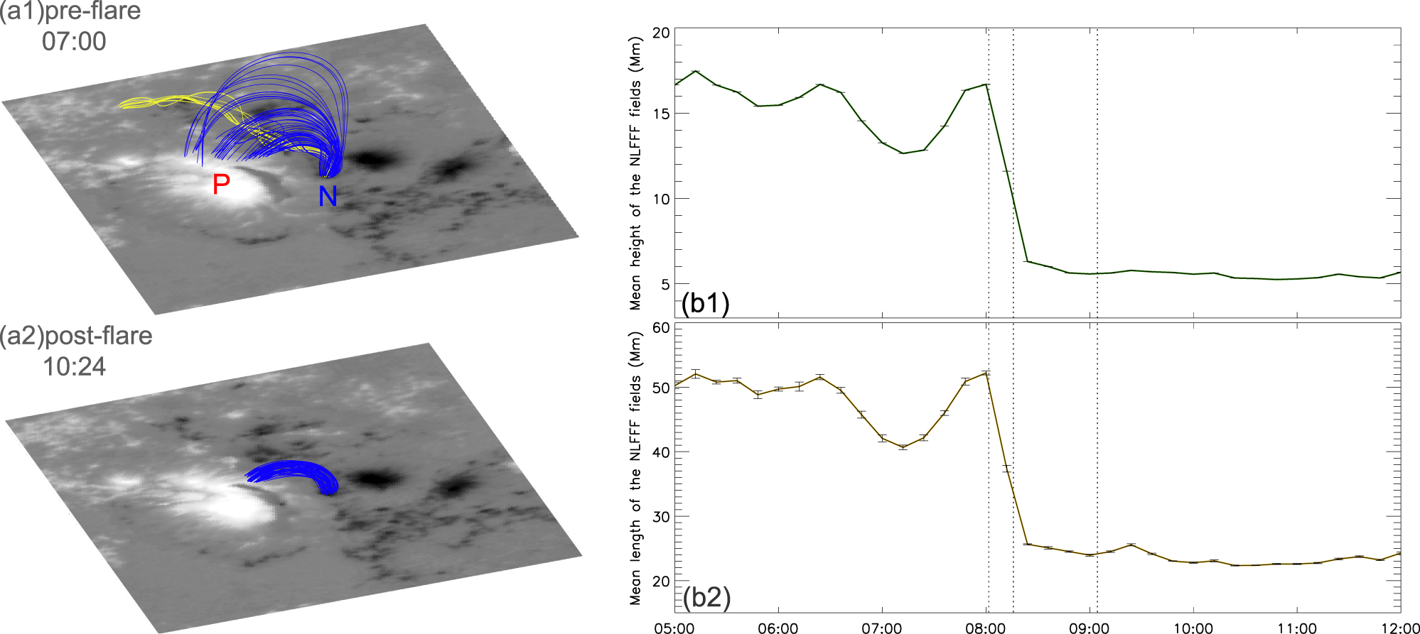
Zoom In Zoom Out Reset image size

Similar to the penumbral reappearance, the sudden motion of umbra provides another excellent example for the photospheric response to the flare eruption. However, more importantly, this sudden moving umbra, considering its strong magnetic field, gives us a more suitable tracer to shed light on the magnetic field reconstruction in the corona. First, the coronal magnetic field ${\boldsymbol{B}}$ can be conducted by the NLFFF extrapolation model (Wheatland et al. 2000; Wiegelmann 2004; Wiegelmann et al. 2006, 2012). Then we concentrate our analysis on a part of the NLFFF model lines that are traced from the region N. In Figure 5, 3D views of these field lines are presented to show the magnetic field configuration before and after the flare (panels (a1)–(a2)). It can be seen that these field lines are divided into two different system. The yellow lines exhibiting a flux-rope characteristic can be regarded as a part of the filament fields, while the blue lines connect to the north of the sunspot P, which constitute a magnetic arch system. Statistically, the magnetic arch system accounts for ∼90% of the whole fields traced from N, the filament system only accounts for ∼1%, and the rest of the lines connected to the other regions are referred to as an unrecognizable part. In order to show more clearly, only magnetic arch and filament fields lines are plotted, and the proportion between the two systems is set to a proper scale. After careful comparison, we find that the magnetic arch fields collapsed down significantly after the flare, with the field lines becoming lower and shorter. In particular, the region right below the collapsing magnetic arch was exactly the area where the penumbral reappearance happened. To verify the temporal relationship between the field contraction and the flare eruption, we performed the extrapolation for every 12 minutes in 7 hr, and randomly picked 1500 field lines traced from the region N 10 times to estimate the uncertainty. The lines belonging to the magnetic arch system are selected for tracking the time profiles of their mean height and length. Obviously, in the results (panels (b1)–(b2)), the mean height of the magnetic arch dropped down significantly and permanently from ∼16.7 Mm to ∼5.6 Mm during the flare. At the same time, the mean length of the field lines decreased from ∼52.2 Mm to ∼24.5 Mm. In light of the above situations, the NLFFF model provides a possible interpretation that the coronal field contraction may lead to photospheric perturbations during the flare.

Zoom In Zoom Out Reset image size

In this Letter, we have presented a detailed analysis of the sudden photospheric variations in the 2015 June 25 M7.9 flare. By using the Hinode G-band and HMI intensity images, we provide the first valid observations of sudden penumbral reappearance and umbral motion during the major flare. To confirm the idea that these changes are the photospheric responses to the flare eruption, we further analyze the photosphere magnetic fields, compute the local LF changes, and investigate the coronal field reconstruction by NLFFF modeling. The main results are summarized as follows.

• 1.  
  In the region around the PIL, the originally decaying penumbra shows a sudden reappearance, with the intensity decreasing abruptly during the flare. Such a feature can be regarded as a reversal signal when the sunspot is in the decline phase, and thus indicates that the penumbral reappearance is probably induced by the eruption in the upper atmosphere.
• 2.  
  The fibrils of the reappearing penumbra are almost aligned in the y direction. Coincidentally, only ${\boldsymbol{B}}$_y of the vector fields in the central PIL region were strengthened rapidly during the flare. Moreover, a downward LF changes appeared indicating that the pressure from the upper atmosphere was suddenly enhanced.
• 3.  
  The umbra of sunspot N suffered a northeastward horizontal LF change during the flare. Meanwhile, a sudden movement can be observed in the same direction. Based on the NLFFF model, we can see that region N is one footpoint of a magnetic arch system, which is connected to the north part of sunspot P. During the flare, the magnetic arch fields collapse down suddenly, and the region right below the magnetic arch is exactly the area where the penumbral reappearance happened.

Hence, a clear and causal picture of this event can be established by the idea of the magnetic implosion and back reaction from coronal field reconstruction. When the magnetic energy releases in the eruption, the upward momentum of the implosion escapes away from the upper coronal fields, and eventually evolves into an asymmetric full CME, whereas the downward momentum pushes the central fields down to lead to the contraction of the magnetic arch. Reflected in the photosphere, the magnetic field along the PIL becomes more inclined, and the local pressure is significantly enhanced after the flare. Consequently, the original decayed penumbra reformed in the region right below the magnetic arch. On the other hand, the field contraction implies a stronger connection between the two footpoints of the magnetic arch, which accounts for the lateral pressure increasing in the umbra region. As a result, the small negative sunspot N shows a sudden transverse movement toward the large positive sunspot P, which is located on the other side of the flaring PIL.

Clearly, the above scenario can well explain the sudden photospheric variations in this event. We can further speculate that different kinds of coronal reconstructions could result in different responses in the photosphere. To confirm this idea, more observations and extended analysis should be investigated in future solar flare research.

We sincerely thank the SDO team and the Hinode team for data support. This work is supported by the Natural Science Foundation of China under grants 11633008, 11473065, 11333007, 11403098, 11503081, and 11633008, and the CAS "Light of West China" Program.