


Abstract
Using data from the Magnetospheric Multiscale (MMS) and Cluster missions obtained in the solar wind, we examine second-order and fourth-order structure functions at varying spatial lags normalized to ion inertial scales. The analysis includes direct two-spacecraft results and single-spacecraft results employing the familiar Taylor frozen-in flow approximation. Several familiar statistical results, including the spectral distribution of energy, and the sale-dependent kurtosis, are extended down to unprecedented spatial scales of ∼6 km, approaching electron scales. The Taylor approximation is also confirmed at those small scales, although small deviations are present in the kinetic range. The kurtosis is seen to attain very high values at sub-proton scales, supporting the previously reported suggestion that monofractal behavior may be due to high-frequency plasma waves at kinetic scales.
Export citation and abstract BibTeX RIS
1. Introduction
A central characteristic of turbulence is the transfer of energy across scales. In quasi-steady conditions this leads to a self-similar distribution of fluctuation energy across an inertial range of scales. During energy transfer, turbulence typically forms coherent structures that concentrate gradients so that dissipation becomes intermittent. This standard picture has been developed based on theory, laboratory experiments, and numerical simulation, for hydrodynamic (Monin & Yaglom 1971, 1975; Sreenivasan & Antonia 1997) and magnetohydrodynamic (Pouquet et al. 1976; Biskamp 2003) models. Extension of these ideas to kinetic space plasmas such as the solar wind has progressed (Tu & Marsch 1995; Yordanova et al. 2009; Matthaeus et al. 2015) through availability of high-resolution spacecraft instrumentation (Alexandrova et al. 2008; Sahraoui et al. 2009; Perri et al. 2012). Studies of solar wind turbulence have recently emphasized a fundamental problem—namely, the manner in which cascaded energy converts into heat at proton and sub-proton kinetic scales (Wan et al. 2012b; Alexandrova et al. 2013; Karimabadi et al. 2013; TenBarge et al. 2013).
The Magnetospheric Multiscale (MMS) mission has instrumental capabilities well suited for addressing such questions (Burch et al. 2016). Small spacecraft separations maintained by MMS are ideally suited to probe kinetic-scale structures. Fine-scale observations employing the familiar Taylor "frozen-in flow" approximation are also supported.
To date, MMS studies have emphasized the primary mission goal of magnetospheric magnetic reconnection. MMS observations in the magnetosheath have also broken new ground in plasma turbulence research (Huang et al. 2016; Yordanova et al. 2016; Chasapis et al. 2017). Here, we directly examine solar wind magnetic turbulence at unprecedented small scales, down to 6 km, deep into the kinetic range approaching electron inertial scales (typically ∼ a few kilometers in the solar wind near 1 au). We examine second-order structure functions evaluated two ways—using the Taylor hypothesis and by direct two-point multi-spacecraft measurements. A similar analysis explores the scale-dependent kurtosis, a statistic that provides a measure of intermittency and coherent magnetic structures. The results (a) confirm directly that nearly power-law energy spectra extend to near electron scales, (b) that the Taylor hypothesis remains approximately accurate to those scales, and (c) that the scale-dependent kurtosis appears to reach very high values approaching electron scales, clarifying earlier results.
2. MMS and Cluster Observations in the Solar Wind
To cover a wide range of spatial lags, we selected five MMS intervals and three Cluster intervals with varying spacecraft separations. The selected intervals are described in Table 1, including time coordinates, spacecraft separation, and plasma parameters: mean magnetic field strength  , the rms magnetic fluctuation
  , mean density
  , ion and electron inertial scales di and de, proton beta
  , Alfvén speed Va, and the solar wind velocity VSW.
Table 1. Description of the Selected Solar Wind Intervals and Relevant Plasma Parameters
| Mission | Date | Time | Separation |

|

|

|
di | de |

|
Va | VSW |
|---|---|---|---|---|---|---|---|---|---|---|---|
| (km) | (nT) |

|
(km) | (km) | (km s−1) | (km s−1) | |||||
| MMS | 2016 Dec 06 | 11:37:34–11:44:03 | 5.89 | 7.30 | 0.30 | 16.2 | 56.6 | 1.3 | 0.3† | 41.3 | 350 |
| MMS | 2016 Dec 09 | 10:47:04–10:50:03 | 5.98 | 7.89 | 0.14 | 6.4* | 89.9* | 2.1 | 3.0* | 68.7* | 624 |
| MMS | 2016 Dec 07 | 14:49:54–14:55:03 | 6.40 | 8.54 | 0.15 | 24.1 | 46.3 | 1.0 | 0.7† | 38.3 | 354 |
| MMS | 2016 Dec 31 | 08:19:54–08:25:03 | 8.05 | 6.31 | 0.05 | 20.2* | 50.7* | 1.2 | 0.3*† | 30.8* | 307 |
| MMS | 2015 Nov 03 | 06:17:34–06:22:33 | 16.67 | 15.36 | 0.07 | 89.2* | 24.1* | 0.6 | 2.6*† | 35.5* | 352 |
| Cluster | 2002 Feb 19 | 01:30:00–02:00:00 | 168.18 | 8.02 | 0.40 | 18.9 | 52.4 | 1.2 | 1.0 | 38.1 | 360 |
| Cluster | 2004 Jan 10 | 07:10:00–07:20:00 | 206.37 | 13.30 | 0.11 | 14.2 | 60.4 | 1.4 | 6.6 | 76.8 | 721 |
| Cluster | 2006 Apr 04 | 19:30:03–20:00:00 | 9811.94 | 8.12 | 0.08 | 9.2 | 75.0 | 1.7 | 0.2 | 59.4 | 316 |
Note. Asterisk denotes intervals where the proton density was considered less reliable, and so the electron density was used to estimate the marked values. Values marked with a dagger denote the intervals where the temperature measurements by FPI were considered unreliable. For those values, the temperature provided by WIND was used. A comparison of MMS and WIND measured parameters is given in the Appendix.
Download table as: ASCIITypeset image
Spacecraft separation for the MMS intervals ranges from 6 to ∼15 km, which is below the solar wind ion inertial length. We used burst-mode resolution data from the MMS flux-gate magnetometer at 128 Hz. The plasma density, temperature, and velocity were provided by the FPI instrument. For comments of data quality, see Table 1 and the Appendix. The Cluster intervals have spacecraft separation from 100 km up to 10,000 km. These intervals, while not tightly controlled (see Table 1), are fairly typical of 1 au solar wind. The statistics we examine are based on increments and are relatively insensitive to large-scale fluctuations, while the kurtosis is a normalized quantity, allowing direct comparison of these intervals. Our choice of intervals enables access to multi-point solar wind turbulence statistics, beginning with the inertial range and extending deep into the kinetic range of scales. For the Cluster intervals we used flux-gate magnetic field data at 22 Hz for the 2002 and 2006 intervals and at 67 Hz for the 2004 interval. Plasma density, temperature, and velocity are from the PEACE and CIS-HIA/CODIF instruments.
3. Calculation of Magnetic Field Increments
Our interest is in high-resolution solar wind data at very small inter-spacecraft separations. This permits analysis of small-scale structures, both directly and through use of the Taylor frozen-in approximation. Such data sets are limited in time duration as the Cluster and MMS spacecraft spend relatively limited time in the pristine solar wind. Therefore, it becomes advantageous to compute statistics in terms of the increments of the magnetic field, rather than statistics of the fields themselves (Monin & Yaglom 1971, 1975). Below, we analyze second- and fourth-order moments based on magnetic increments.
Let  represent the magnetic field vector, a function of space and time. For single-spacecraft analysis the time increments of magnetic field are defined as

where it is understood that the field is evaluated at a single-spacecraft position, viewed here as fixed in space, and τ is the time lag. For the single-spacecraft case we employ the Taylor hypothesis in approximating spatial statistics. At a formal level this is implemented by treating the time increment as equivalent to a spatial increment in the "frozen-in" medium.
For the two-spacecraft case, we designate the magnetic field increment as

where t is the time of each measurement, and the pair of indices i, j = 1, 2, 3, 4 correspond to a pairing of two of the four MMS spacecraft. In this case, the increment is associated with a spatial separation  where
where  and
and  are the positions of the ith and jth spacecraft. Note that the frequency response of MMS/FGM is adequate to resolve the high-cadence signal we employ (Russell et al. 2016), while the stability of intercalibration of the four MMS magnetometers was found to be satisfactory for the increments computed here.
4. Structure Functions and Accuracy of the Taylor Hypothesis
The second-order spatial structure function of the vector magnetic field may be defined in the usual way (Monin & Yaglom 1971, 1975) as

where the magnetic field  is evaluated at two distinct points separated by a vector lag
  , and both values of the magnetic field are evaluated at the same instant of time t. For a statistically homogeneous medium,
  is independent of
  . If the turbulence is stationary in time and ergodic (Monin & Yaglom 1971, 1975) then the ensemble average
  may be approximated by averaging over time t at fixed spatial lag.
With these preliminaries, the evaluation of  proceeds employing the approaches suggested by Equations (1) and (2).
For the single-spacecraft evaluation we compute

using time-lagged increments in the sense of Equation (1) and averaging the squared vector increments over a suitably long time interval T. Here, Vsw is the average solar wind speed in the interval, provided by the electron velocity measurements, and  is a radial unit vector. We note that for relatively large values of T (i.e., above
  ), the estimated value of
  has no significant dependence on the averaging interval T. Hence, for each case the averaging interval T is the full size of the data sample, as noted in Table 1.
For the two-spacecraft evaluation we compute  for the six distinct pairings (i, j) of the four spacecraft. For this case,


where t is measurement time and again  label the four MMS spacecraft. Note that the structure functions of the vector
  may also be decomposed into scalar structure functions from each component, but this is not pursued here.
To interpret the structure functions, we briefly recall their familiar relationships with correlation functions and spectra. The two-point correlation function of the random, statistically homogeneous vector field  is
is  , which is related to the structure function by
  . The wavenumber (
 ) spectrum is
  . Integrating over all directions gives the Kolmogorov omnidirectional spectrum E(k), which for strong hydrodynamic turbulence is
  in the inertial range. It is interesting to note that in the inertial range of scales, the quantity
  behaves as an "equivalent spectrum" viewed as a function of an effective wavenumber
  . If there is a power-law range
  of sufficient bandwidth, we expect to find
  over a similar range of
  . This holds at least for
  . This relationship is clearly useful for analysis of the structure functions, but it is important to emphasize that
  is not identical to the spectrum, and k* is not the wavenumber k.
Figure 1 illustrates the structure functions for the selected intervals, shown as equivalent spectra. The Cluster intervals supply the larger spacecraft separations, while the small separation of the MMS spacecraft allows estimates of the structure functions well into the kinetic range. The structure functions are computed from both methods described above. First, we use the Taylor hypothesis as in Equation (4), which is shown as four lines on Figure 1 from each of the four spacecraft. Second, direct two-spacecraft increments are employed to compute D(2), as in Equation (6). These results are shown as six individual points on Figure 1 for each pair of spacecraft.
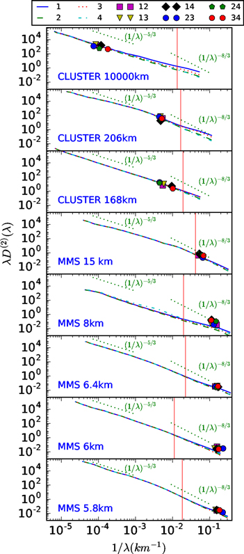
Figure 1. Second-order structure functions from Cluster and MMS vs. spatial lag λ, computed (a) directly from two-spacecraft measurements (symbols) and (b) from single-spacecraft measurements using the Taylor hypothesis (lines). The characteristics of the selected intervals shown here are described in Table 1. The top three panels show the results obtained from Cluster observations at spacecraft separations ranging from ∼10,000 km down to ∼100 km. The bottom five panels show the MMS observations at spacecraft separations ranging from ∼6 km to ∼15 km. Vertical solid line indicates the ion inertial scale di.
Download figure:
Standard image High-resolution imageIt is apparent in Figure 1 that there is a broad agreement between the multi-spacecraft calculations and those based on the Taylor hypothesis. Moreover, the general picture of a Kolmogorov −5/3 inertial range giving way to a steeper (∼−7/3 or −8/3) kinetic/dispersion range is generally consistent with observational (Alexandrova et al. 2008; Sahraoui et al. 2009) and theoretical (Boldyrev et al. 2015) studies that examine this issue in detail.
It is noteworthy that a small systematic discrepancy between the direct estimates and the Taylor-based estimates appears to emerge at the smallest spatial scales. In particular, the two-spacecraft measurements have consistently larger values of structure function at those scales, which can be somewhat counterintuitive. For stationary and homogeneous samples one would expect that the variance at a given scale would be larger when inferred from the Taylor hypothesis. This is expected because the single-spacecraft estimate includes the variance due to undistorted propagation over a distance equal to the spatial lag and, in addition, a contribution due to the time variation during the time of passage of that distance. In fact, this systematic difference, on average, forms the basis for estimating the Eulerian decorrelation time (Weygand et al. 2013) when data from multiple spacecraft are available.
At these very small scales, it appears that this reasoning may fail. In fact, a small systematic elevation of the variance in the two-spacecraft estimates relative to the one-spacecraft Taylor estimates occurs in Figure 1 in all of the very small separation MMS observations.
The standard reasoning actually relies on the two-spacecraft estimate being sufficiently averaged so that the statistics become homogeneous in space. Evidently, what is happening here is that there are structures (strong gradients) present between spacecraft that contribute to the increments, but these do not affect the Taylor single-spacecraft estimates that can be affected only by gradients in the direction of the plasma flow.
Figure 2 quantifies the small differences between the single-spacecraft and the two-spacecraft results. Smaller values, those located near the lower left corner of the plot, correspond to smaller spatial separations. Here, we can see that the fine-scale structures that cause the effect alluded to above are having a more pronounced influence at very small scales. At the large spacecraft separations the distribution of points is more symmetric, consistent with what has been observed at much larger scales, e.g., in Weygand et al. (2013).

Figure 2. Comparison of second-order structure function computed directly using two-spacecraft measurements (horizontal axis) and estimated from single-spacecraft measurements using the Taylor hypothesis (vertical axis) for each interval. The solid black line denotes a slope of 1 where the two values are equal. Each of the 6 multi-spacecraft values is plotted against the two corresponding single-spacecraft values.
Download figure:
Standard image High-resolution image5. Scale-dependent Kurtosis and Kinetic-scale Intermittency
Higher-order statistics provide insights concerning structure and intermittency in turbulence, in effect emphasizing the tails of underlying distribution functions. Of particular importance is the kurtosis, or normalized fourth-order moment, for varying spatial lag. This scale-dependent kurtosis, for the increment of the vector magnetic field, is defined as

A large kurtosis κ at a given lag indicates that increment takes on large values with elevated likelihood, producing a non-Gaussian distribution. It also indicates that the large values of that increment occur in limited regions of space, corresponding to the useful heuristic interpretation that the kurtosis is of the order of the reciprocal of the fractional volume filling factor.
Like the second-order structure functions, the scale-dependent kurtosis may also be estimated either using two-spacecraft increments, as in Equation (2), or using single-spacecraft increments, as in Equation (1).
In the former case,

and in the latter,

where the spacecraft indices  , the averaging interval T, and time lag τ are the same as previously defined.
Figure 3 shows the scale-dependent kurtosis  for both methods. Note that the results are plotted against the magnitude of the lag, so that the direction of the vector lag is not taken into account. The lag is normalized to the ion inertial scale di. It is apparent that at larger lags,
  , the value of κ increases as lag decreases. This is typically viewed as a signature of intermittency (Frisch 1995). Such behavior is typically observed and is usually identified with a multi-fractal interpretation of the intermittency, in the inertial range of both hydrodynamics (Anselmet et al. 1984) and MHD (Biskamp 2003). However, for plasmas it also has been noted (Sundkvist et al. 2007; Leonardis et al. 2013; Wu et al. 2013) that near scales of a few di and smaller, one may find a flattening of κ, or even a decrease, as one moves toward smaller lags. This is seen in both observations and kinetic simulations (Wan et al. 2012a; Wu et al. 2013), although various observational limitations and possible noise signals have confounded a clear interpretation. One possibility is that kinetic turbulence becomes monofractal at sub-proton scales (Leonardis et al. 2013). Another explanation might be that plasma waves, even with relatively small amplitudes, can destroy coherence and halt the increase of phase correlations at smaller kinetic scales (Wan et al. 2012a).

Figure 3. Scale-dependent kurtosis directly computed from two-spacecraft measurements (symbols) and from single-spacecraft measurements using the Taylor hypothesis (lines). The shaded regions show the spread of the four single-spacecraft estimates, and the line is their average value at each scale. Different colors are used for the different intervals. There is a general increase as the lag decreases toward a few di. However, at di and below, the single-spacecraft estimates decrease, while the two-spacecraft estimates attain large values as the lag decreases to ∼6 km.
Download figure:
Standard image High-resolution image
As is evident in Figure 3, this change in behavior for lags less than a few di is also seen here in the single-spacecraft estimates. It should be noted that most previous reports of this sort of behavior also employed the Taylor hypothesis.
However, the two-spacecraft results for κ that are shown here behave differently. In fact, at the smallest scales, the two-spacecraft MMS results at ∼6 km separation yield a varying kurtosis that can be as large as 100. This may be due to very sharp coherent structures that have specific orientation relative to the MMS inter-spacecraft baselines.
This observation implies that it is possible to see very large kurtosis at scales approaching the electron scales, which has not been observed before. It is noteworthy that the decrease in κ toward the small scales occurs for single-spacecraft results that depend on the Taylor hypothesis. One interpretation is that the intrinsic time dependence, neglected in the Taylor hypothesis, begins to have a significant effect at those small scales. This is consistent with the view (Wan et al. 2012a) that short-wavelength high-frequency fluctuations are present at sub-proton scales, leading to time dependence that obscures the coherence needed for large κ.
6. Discussion
This Letter presents an analysis of a selection of solar wind observations from the Cluster and MMS missions, including single-spacecraft and two-spacecraft statistics focusing on second- and fourth-order statistics, namely, structure functions and scale-dependent kurtosis. These analyses were able to confirm several key properties, examining them here at unprecedented small scales ∼6 km, well into the kinetic range and approaching the electron inertial scale. The main results are (i) that the standard power-law and spectral break in the (equivalent) spectrum persists at sub-proton scales, deep into the kinetic range; (ii) that the Taylor frozen-in flow approximation appears to remain generally valid down to those small scales; and (iii) that the scale-dependent kurtosis, directly measured using two-spacecraft measurements, attains large values for lags approaching electron scales, while the single-spacecraft result shows a decrease at scales smaller than ion scales.
These results demonstrate the capabilities for exploring new space plasma physics and plasma turbulence parameters regimes when data are available from a multi-spacecraft mission such as MMS, with small inter-spacecraft separations and high-resolution instrumentation.
At very small, sub-proton scales we identified discrepancies between the two-spacecraft results and the single-spacecraft results. We attributed the higher (increment) variances observed in the two-spacecraft statistics to the presence of sub-proton scale spatial structures (see, e.g., Perri et al. 2012; Karimabadi et al. 2013), evidently anisotropic in nature, that are undetected by the single-spacecraft analysis that relies on the Taylor approximation. We also observed a striking difference at very small scales in the behavior of the scale-dependent kurtosis. Once again the direct two-spacecraft estimates signaled the presence of highly coherent spatial structures, as the kurtosis reached values ∼100 or more. However, the single-spacecraft analysis data, which are sensitive to time variations, do not detect these structures, possibly due to high-frequency waves. Both of these results add to accumulating evidence of the importance of coherent structures at sub-proton kinetic scales, while also at least partially clarifying prior results (Sundkvist et al. 2007; Wan et al. 2012a; Leonardis et al. 2013; Wu et al. 2013).
Future observations by the MMS spacecraft in the solar wind, during the upcoming phases of the mission, will provide a unique opportunity to further study these questions.
This research partially supported by the MMS mission through NASA grant NNX14AC39G, and in part by NSF-SHINE AGS-1460130 and the NASA Helio-GI program grant number NNX17AB79G, all at the University of Delaware. A.C. is supported by the NASA grant. W.H.M. is a member of the MMS Theory and Modeling team. We would like to acknowledge the assistance of the MMS instrument teams, especially FPI and FIELDS, in preparing the data, as well as the work done by the SDC. The data used in this analysis are Level 2 FIELDS and FPI data products, in cooperation with the instrument teams and in accordance their guidelines. All MMS data are available at https://lasp.colorado.edu/mms/sdc/. The Cluster data were provided by the Cluster Science Archive https://www.cosmos.esa.int/web/csa.
Appendix: Measurements of Solar Wind Parameters
Table 2 compares the average values of the electron and proton moments as measured by the electrostatic analyzers of the FPI instrument of MMS and proton moments measured by the Faraday cups of the SWE instrument of WIND for each interval. In some instances, the proton density ni and the electron Te and proton Ti temperature measured by the FPI instrument on MMS were found to be less reliable. Densities ne and ni are shown in cm−3, temperatures Te or Ti in eV, and velocities Ve and Vi in km s−1. Subscripts indicate electrons e and protons i.
Table 2. Comparison of Solar Wind Plasma Measurements from MMS and WIND
| Interval | MMS | WIND | MMS | WIND | MMS | WIND | ||||
|---|---|---|---|---|---|---|---|---|---|---|
| Date | Time | ne | ni | ni | Te | Ti | Ti | Ve | Vi | Vi |
| 2016 Dec 06 | 11:37:34–11:44:03 | 17.3 | 16.2 | 13.0 | 11.1 | 15.4 | 2.4 | 426 | 350 | 356 |
| 2016 Dec 09 | 10:47:04–10:50:03 | 6.4 | 9.5 | 5.7 | 13.5 | 74.4 | 34.3 | 666 | 624 | 629 |
| 2016 Dec 07 | 14:49:54–14:55:03 | 25.9 | 24.1 | 23.2 | 19.3 | 17.6 | 4.4 | 354 | 354 | 359 |
| 2016 Dec 31 | 08:19:54–08:25:03 | 20.2 | 13.5 | 23.2 | 11.7 | 12.4 | 1.2 | 365 | 307 | 311 |
| 2015 Nov 03 | 06:17:34–06:22:33 | 89.2 | 48.6 | 146.7 | 13.2 | 20.1 | 8.1 | 405 | 352 | 404 |
Download table as: ASCIITypeset image