


Abstract
Using the recently extended 2D improved Particle Acceleration and Transport in the Heliosphere (iPATH) model, we model an example gradual solar energetic particle event as observed at multiple locations. Protons and ions that are energized via the diffusive shock acceleration mechanism are followed at a 2D coronal mass ejection-driven shock where the shock geometry varies across the shock front. The subsequent transport of energetic particles, including cross-field diffusion, is modeled by a Monte Carlo code that is based on a stochastic differential equation method. Time intensity profiles and particle spectra at multiple locations and different radial distances, separated in longitudes, are presented. The results shown here are relevant to the upcoming Parker Solar Probe mission.
Export citation and abstract BibTeX RIS
1. Introduction
In large gradual solar energetic particle (SEP) events, protons and ions are accelerated to over several hundred MeV/nucleon in energy. It has been largely accepted that energetic particles in these events are accelerated via the diffusive shock acceleration (DSA) mechanism at the shock fronts driven by coronal mass ejections (CMEs).
Applying DSA to interplanetary shocks and CME-driven shocks has been widely investigated. For example, Lee (1983) solved the coupled particle transport and upstream Alfvén wave intensity equations at a quasi-parallel shock. Using this approach, Gordon et al. (1999) examined particle acceleration at the Earth's bow shock and interplanetary shocks. This was further extended by Lee (2005), who employed a two-stream approximation for the energetic particles. Using same set of equations as Lee (1983, 2005), Ng et al. (2003) solved the time-dependent wave transport equation explicitly, obtaining a time-dependent wave action and energetic particle spectrum. In contrast, Zank et al. (2000), Rice et al. (2003), and Li et al. (2003, 2005) adopted the steady-state DSA solution at different times for a shock propagating through the interplanetary solar wind. At any given time, they adopted the steady-state power-law spectrum for the particles. The maximum particle energy at any given epoch was found by balancing the shock dynamic timescale with the particle acceleration timescale. This approach is particularly appealing for numerical modeling of CME shocks since the analytical power spectrum is only determined by the characteristics of the shock at that time. The model developed first by Zank et al. (2000), and later extended by Rice et al. (2003) and Li et al. (2003, 2005), was call the Particle Acceleration and Transport in the Heliosphere (PATH) model. The CME-driven shock in the PATH model is assumed to be 1D only, and all physical quantities depend only on radial distance. Modeling specific SEP events using the PATH model has been performed by Verkhoglyadova et al. (2009, 2010).
With the STEREO mission and the coming Parker Solar Probe mission, a single SEP event will be observed by multiple spacecraft. Indeed, recent observations (e.g., Cohen et al. 2014; Dresing et al. 2014; Gómez-Herrero et al. 2015) have shown that the longitudinal spreading of SEPs in gradual and impulsive SEP events can be very extended. This could be due to both an extended shock surface and cross-field diffusion. Clearly, to understand multiple spacecraft observations one needs to consider particle acceleration and transport in a two-dimensional model. Extending the PATH to a 2D model has recently been accomplished (Hu et al. 2017). The model, named improved Particle Acceleration and Transport in the Heliosphere (iPATH), has two major improvements over the PATH model: (1) the solar wind and the CME-driven shock are modeled using a two-dimensional MHD code, allowing us to study the longitudinal character of particle acceleration at the CME-driven shock; (2) a refined 2D onion shell module that treats the acceleration process in 2D is used, and (3) an improved transport module that uses the backward stochastic differential equation method has been incorporated and includes both parallel diffusion and cross-field diffusion.
With these improvements, the iPATH model is ideally suited to model a single SEP event from multiple vantage points. Note, however, there are limitations for the iPATH model. For example, the model only addresses that part of a gradual event prior to the shock arrival, and the calculated onsets are based on a shock model starting at 10 Rs. In many large SEP events, and especially ground level enhancement events, the shocks start at lower heights.
We model an example SEP event and obtain the time intensity profiles and particle spectra at multiple longitudes and heliocentric distances. Specifically, we obtain these spectral and intensity profiles for the seven locations shown in Figure 1.
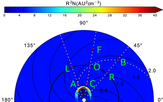
Figure 1. Cartoon showing the configuration for our model calculation. Points L, O, and R are located at 1 au, but separated in longitude. Points C, O, and F are along the same radial direction, and points A, O, B are along the same Parker spiral. See the text for details.
Download figure:
Standard image High-resolution imageThese locations in Figure 1 are chosen such that: (1) points C, O, and F are along a radial direction with a longitude 80°, and heliocentric distances 0.5, 1.0 and 1.5 au, respectively; (2) points A, O, and B are along the same Parker magnetic field line at heliocentric distances 0.5, 1.0 and 1.5 au, respectively; and (3) points L, O, and R have the same radial distance of 1 au, but are separated longitudinally by ±30° s. Our choice of configuration reflects observations made by the current STEREO mission and in anticipation of those to be made by the Parker Solar Probe mission.
We assume that the background solar wind is in steady state with the interplanetary magnetic field, which is given by a Parker spiral,
In this work, we set the solar wind speed to be 400 km s−1 at 1 au. For the total magnetic field strength and proton number density, we use 5.2 nT and 5.67 cm−3 at 1 au. These correspond to observational values averaged over the entire solar cycle 24.
We model the CME-driven shock structure by perturbing the inner boundary at 10 Rs. The simulation runs on a 2D domain with 2000 grid points in the r-direction (from 0.05 to 2.0 au) and 360 grid points in the ϕ direction (not counting the ghost cells). The initial CME speed is set to be 1500 km s−1. The injection efficiency for a strong parallel shock is assumed to be 0.1%. For details of the model, the readers are referred to Hu et al. (2017). In modeling the longitudinal spreading of an SEP event, a key parameter is the perpendicular diffusion coefficient κ⊥ for the energetic particles. Hu et al. (2017) used the Non-Linear Guiding Center theory and calculated particles' perpendicular diffusion coefficient κ⊥ from  (appearing as Equations (12) and (28)). We, however, ignored the radial dependence of l2D in the Equation (12) and assumed a
  . More generally, l2D can have a radial dependence. For example,
  with α in the range of 0–1 (Adhikari et al. 2017; Zank et al. 2017; Zhao et al. 2017). We anticipate that the Parker Solar Probe mission may provide more information on the radial dependence of these two values. With these assumptions, the ratio of κ⊥ to
  used in Hu et al. (2017) can be explicitly expressed as
In this Letter, we set the total turbulence level  to be 0.5 at 1 au and α to be 0. This gives us a
  of 0.018 at 1 au and 0.031 at 0.2 au, for a 10 MeV proton. We find that the simulation results do not strongly depend on the choice of α (using a value of 3/4 for α yields almost the same intensity profiles). Instead, the absolute value of
  affects the simulation results more. See below for details.
2. Simulation Results and Discussion
Figure 2 plots the time intensity profiles prior to the shock arrival as observed at points A, O, and B. These points are along the same Parker field line and so have the same magnetic connection. The solid (dashed) red curve is the time intensity profile of the 4.4 (46.4) MeV particles at point A with r = 0.5 au. The solid (dashed) black curve is the time intensity profile of the 4.4 (46.4) MeV particles at point O with r = 1.0 au. The solid (dashed) blue curve is the time intensity profile of the 4.4 (46.4) MeV particles at point B with r = 1.5 au. The vertical dashed lines mark the shock arrival times at the different locations. At the beginning of the CME, these three points are connected to the western flank of the shock. As the CME propagates out, the connection moves to the nose of the CME. Note that point A has a radial distance of r = 0.5 au and is always connected to the western flank of the CME-shock until the shock passes. In comparison, while point O initially connects to the western flank of the shock, it connects to the shock nose when the nose reaches ∼0.7 au. Afterward, it connects to the eastern flank of the shock. This is also true for point B. Indeed, by the time the shock reaches point B, it corresponds to the very eastern flank of the shock.

Figure 2. Time intensity profiles at locations A, O, and B as shown in Figure 1. These three points are along the same Parker field line. In the right panel, the κ⊥ is five times larger than that in the left panel.
Download figure:
Standard image High-resolution imageBecause these three points are on the same field line, the time intensities for these three points are similar. Consider the 46.4 MeV particles (dashed lines): for all three locations, we see a very fast initial rise, followed by a plateau-like period. For point A, this plateau-like period lasts till the shock arrival. For points O and B, the plateau-like periods are followed by slow decays. We can also see that the SEP onset time is earlier when the point is closer to the Sun. The time intensities for the case of 4.4 MeV are similar to those of the 46.4 MeV case, except that the decays occur at later times. This reflects the fact that the shocks can accelerate particles to 4.4 MeV over a longer time than they can to 46.4 MeV.
Shown in the right panel is the same simulation, but the κ⊥ is increased by a factor of 5. This increase affects the initial phase more. With an enhanced κ⊥, particles accelerated at different part of the shock can now all propagate to any given points (e.g., A, B, or O). We therefore see a faster increase of the time intensity profile. For example, the 4.4 MeV proton observed at 1 au now quickly rises to the peak value at around t = 10 hr and then gradually decays. This is compared to the original case (left panel) where the peak occurs at t = 25 hr. This illustrates how the result can be sensitive to the κ⊥ value.
Figure 3 plots the time intensity profiles prior to the shock arrival as observed at points L, O, and R, which are all located at 1 au but at different longitudes. Such a configuration corresponds to, for example, STEREO-A, STEREO-B, and ACE all observing the same SEP event. In our simulation, point L has a longitude of 110°, point O has a longitude of 80°, and point R has a longitude of 50°. As in Figure 2, the vertical dashed lines mark the shock arrival times at the different locations. The solid (dashed) blue curve is the time intensity profile of the 4.4 (46.4) MeV particles at point L with ϕ = 110°; the solid (dashed) black curve is the time intensity profile of the 4.4 (46.4) MeV particles at point O with ϕ = 80°; the solid (dashed) red curve is the time intensity profile of the 4.4 (46.4) MeV particles at point R with ϕ = 50° au.
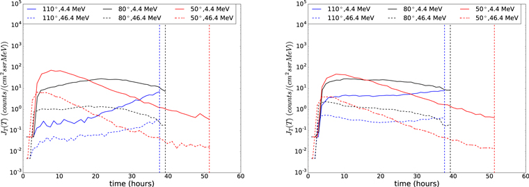
Figure 3. Time intensity profiles at locations L, O, and R as shown in Figure 1. The three locations have the same heliocentric distance of 1 au, but differ in longitude. In the right panel, the κ⊥ is five times larger than that in the left panel.
Download figure:
Standard image High-resolution imageThe time intensity profiles for these three locations differ considerably. Point R connects to the shock nose early on and sees a fast rise, followed by a fast decay, indicating that the magnetic connection moves to the eastern flank of the shock. At location O (base location), the magnetic connection was maintained to the shock nose region for a long duration, therefore the time intensity shows a reasonably fast rise and then maintains a plateau-like feature. In comparison, at location L, the time intensity profiles show very gradual increases with no decay phase. This is because the magnetic connection at point L was initially to the western flank of the shock, and it moves toward the shock nose. However, because the nose of the shock moves along a longitude of 100°, point L never connects to the shock nose before the shock arrival.
Again, shown in the right panel is the same simulation but the κ⊥ increased by fivefold. As explained before, we see a faster initial increase of the time intensity profile.
Figure 4 plots the time intensity profiles prior to the shock arrival as observed in points C, O, and F, which are along a radial direction with a longitude of 80°. As in Figure 2, the vertical dashed lines mark the shock arrival times at different locations. The solid (dashed) red curve is the time intensity profile of the 4.4 (46.4) MeV particles at point C with r = 0.5 au; the solid (dashed) black curve is the time intensity profile of the 4.4 (46.4) MeV particles at point O with r = 1.0 au; the solid (dashed) blue curve is the time intensity profile of the 4.4 (46.4) MeV particles at point F with r = 1.5 au. Because points O, C, and F are located at different distances and on different field lines, we expect the time intensity profiles in this figure to be a mix of those in Figures 2 and 3. However, as seen from Figures 2 and 3, the time intensity profile is mostly determined by the magnetic field line that the observer is on, making Figure 4 more similar to Figure 3. Consider the 46.4 MeV particles. Point C (red curve) shows a very fast rise, followed by the fastest decay. This of course is because point C is connected to the shock nose early on and the connection quickly moves to the eastern flank of the shock, where particle acceleration is less efficient. In comparison, the initial rise at O is slower and that at F is the slowest. Again, shown in the right panel is the same simulation but the κ⊥ increased by fivefold. As explained before, we see a faster initial increase of the time intensity profile.
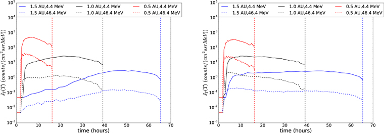
Figure 4. Time intensity profiles along one radial direction (with the same longitude of 80°) for points C, O, and F as shown in Figure 1. In the right panel, the κ⊥ is five times larger than that in the left panel.
Download figure:
Standard image High-resolution imageFigure 5 plots time-integrated spectra at all seven points. For each spectrum, the integrated time is from the beginning of the event until the shock arrival at that location.

Figure 5. Event-integrated spectra for different configurations. The left panel is for points along the same field line: A, O, and B; the middle panel is for points at 1 au but with different longitudes: L, O, and R; the right panel is for points along the radial direction: C, O, and F. See the text for more details.
Download figure:
Standard image High-resolution image
The left panel is for locations along the same field line: the red curve for location A, black for location O, and blue for location B. As we can see, the shapes of the event-integrated spectra along the same field line are similar. The magnitude of the event-integrated fluences decreases with increasing distance. At 10 MeV, the fluence at r = 1.5 au is over 10 times smaller than that at r = 0.5 au. The middle panel is for locations at the same r = 1 au, but with different longitudes: the blue curve is for location L, black for location O, and red for location R. The shapes of the event-integrated spectra at these three locations are different. The magnitudes also differ. The fluence at location L is an order of magnitude smaller than those at locations O and R. Consequently, the same SEP event, as observed at different longitudes will prompt different space-weather concerns. The right panel is for locations O, C, and F, which are along the same radial direction. In this case, both the magnitudes and the maximum energies are different. The maximum energies are different because the maximum energies were accelerated at different shock locations (i.e., different longitudes). The magnitudes are different mainly because they are measured at different distances (see also Verkhoglyadova et al. 2012).
3. Conclusion and Discussion
In this Letter, we examine time intensity profiles and particle spectra at multiple observational locations for an example gradual SEP event using the iPATH model. With the existing STEREO spacecraft and the upcoming Parker Solar Probe mission, observations of a single SEP event at multiple places will become common. However, simulations of a single SEP event at different locations are still scarce. Previous simulations have focused on studying the time evolution and particle spectra at a single observation point. More recently, recognizing the importance of cross-field diffusion, Qin et al. (2013) have examined the transport of SEPs in large SEP events. However, in that work, particle acceleration is treated in an ad hoc manner and the accelerated particle source at the shock is assumed to be of a very simplified form. The iPATH model, which we recently extended from its predecessor, the PATH model, considers both particle acceleration at a 2D moving shock and the subsequent particle transport in the heliosphere. In this Letter, using the iPATH model, we obtain time intensity profiles and particle spectra at different places that vary in both radial distance and longitude. As an intrinsic 2D model, the iPATH model provides a working basis to interpret multi-spacecraft observations of a single SEP event. This is of particular importance to simultaneous ACE and STEREO observations of a single SEP event where the spacecraft have a large separation in longitude. Furthermore, it is also important for future simultaneous observations by ACE, Parker Solar Probe, and Solar Orbiter where both the heliocentric distance and the longitudes of the spacecraft differ.
We note that the iPATH model treat the CME and its driven shock in a manner, although similar to the WSA-ENLIL+Cone model, very simplified. A proper treatment of the CME, for example, as those adopted in Feng et al. (2011, 2012) and Jin et al. (2013), can conceivably yield more realistic CME and therefore CME-driven shock descriptions (such as the shock width, shock compression ratio, and shock geometry, etc.). However, since the time intensity profiles and particle spectra in the iPATH model only depend on the shock parameters, not those of the CMEs, we expect that, as long as the shock model in the iPATH resembles those from a more realistic CME model, the results would not change much. Nevertheless, employing a more realistic CME model in the iPATH will mark a significant step forward in understanding SEP events.
This work is supported at UAH by a NASA grant NNX15AJ93G. G.P.Z. also acknowledges the partial support of the Parker Solar Probe mission through a subcontract SV4-84017 from the JHU/APL contract 975569.