
Abstract
Some aspects of the thermodynamics and mechanics of solid surfaces, in particular with respect to surface stress and surface energy, are reviewed. The purpose is to enlighten the deep differences between these two physical quantities. We consider successively the case of atomic flat surfaces and the case of vicinal surfaces characterized by surface stress discontinuities. Finally, experimental examples, concerning Si surfaces, are described.
Export citation and abstract BibTeX RIS

Content from this work may be used under the terms of the Creative Commons Attribution 3.0 licence. Any further distribution of this work must maintain attribution to the author(s) and the title of the work, journal citation and DOI.
1. Introduction
Surfaces and thin films are becoming increasingly important in nanoscience and nanotechnology. In this context, understanding surface elasticity has been recognized as an important challenge [1, 2], especially in the field of nanomechanics [3, 5]. In recent decades surface elasticity has thus been extensively studied with a special emphasis on surface stress concept [1–5] and elastic interaction between steps on a surface [5–7]. The purpose of this short invited review is to clarify some misinterpretations that can still be found in the recent literature in spite of many recent improvements [8–12]. Moreover, we take the opportunity of this invitation to synthesize several results obtained by our group in Marseille but scattered in several different papers [2, 4, 5, 13–16].
2. The surface stress concept
2.1. The mechanical approach
Classical theory of elasticity treats solids as continuum mediums. Let us consider a piece of matter (of volume V limited by a surface S) in an infinite body. This volume is submitted to two forces fields: the forces  exerted by the remaining body on the surface boundary of the piece of matter and the external forces
  originating from an external field such as, for instance, gravity. At equilibrium, these forces are written as
  and
and  , where σij are the components of the bulk stress tensor and n is a normal unit vector directed towards the exterior of the surface. The virtual work against an infinitesimal displacement field δu can thus be written
  . Using the above-mentioned equilibrium expressions of fisurf and fiext and the divergence theorem to transform the surface integral to an integral on the whole volume, there is [2, 17]

This elastic energy is an extensive quantity. As described by Gibbs [18], any extensive quantity may present an excess at the interface between two materials. When one of the materials is in vacuum, this excess quantity is a pure surface-excess and is defined as the difference between the energy of the whole system (bulk + surface) minus the energy of a piece of bulk having the same volume (without surface). In the case under study we can thus define the surface elastic energy as

where σij (z) and εij (z) are the true stress and strain profiles for the complete system (bulk + surface), whereas σijB and εijB are the homogeneous stress and strain tensors in the homogeneous bulk. When considering mechanical equilibrium and non-gliding conditions this equation can be simplified [2]:

where

defines the quantity sα β as an excess quantity of the bulk stress component tangential to the surface [1, 2]. This quantity is thus called surface stress3. Surface stress components may be positive (tensile) or negative (compressive). Obviously for an isotropic surface sα β = sδα β where δα β is the Kronecker symbol.
For illustrative purposes, figure 1 shows the calculated energy versus normal deformation εzz (figure 1(a)) and versus in-plane deformation εxx (figure 1(b)). Three calculations have been performed [2]: for a bulk material, for an un-relaxed slab of n layers then for an elastically relaxed slab. The calculation has been performed using the Wien2k code [20] (ab initio calculations by Wien code for a cubic material). For the slab, two calculations have been performed, the first one is for an un-relaxed slab the second one for a relaxed slab.

Figure 1. (a) Elastic energy versus strain εzz for a bulk material (circles), an unrelaxed slab (squares) and a relaxed slab (diamonds). (b) Elastic energy versus strain εxx for a bulk material (circles), an unrelaxed slab (squares) and a relaxed slab (diamonds). Note that when the elastic relaxation of the slab is properly taken into account, the parabola Δ E(εxx ) is shifted but not for the parabola Δ E(εzz ). It means that the components siz = 0.
Download figure:
Standard image High-resolution imageFigure 1 shows that (i) for such small deformations Hooke's law is valid (quadratic shape of the bulk energy), (ii) for an unrelaxed slab, the surface stress shifts the parabola of the bulk energy and (iii) for an elastically relaxed slab, the bulk parabola is shifted for the in-plane deformation but remains centred on zero for the normal deformation. This last point (iii) simply illustrates that, at mechanical equilibrium, surface stress components siz must be zero so that surface stress can be considered as a degenerated two-dimensional second rank tensor (in the referential of the flat surface)

2.2. The thermodynamic approach
For fluids, first and second principles lead to the classical expression of the differential of the internal energy change

where S, V, Ni, T, P and μi are the usual thermodynamics quantities entropy, volume, number of atoms, temperature, pressure and chemical potential of species i.
The internal energy U(S,Ni ,V) is a homogeneous function of first order so that equation (6) can be integrated by means of the Euler procedure giving thus

For solid systems containing surfaces, the analogue of equations (6) and (7) has to be found [2, 21–24].
Let us consider, at first, the differential of the superficial energy change due to a change of heat, a change of the number of surface particles and a surface area change dA. It is tempting to write

However, since the days of Gibbs [18] it is known that the surface area can be changed by two different processes: creation at constant strain or deformation at constant number of surface atoms. The isothermal work to create a surface at constant strain reads dWcre = γ dA (where the quantity γ is connected to the surface energy density fsurf by fsurf = γ - Nisurf μi /A ), whereas the isothermal work necessary to deform a surface at a constant number of surface atoms obtained in equation (3) can be written  where A0 is the undeformed surface area and dεα β the bulk strain extrapolated to the surface).
Expression (8) is thus difficult to use since g dA has to be identified to γ dAdef or  according to the thermodynamic transformation that is considered. Obviously, one can imagine a process in which there is surface creation and surface deformation so that from a general viewpoint g in (8) is defined by

Obviously g dA has no physical meaning and cannot be measured, whereas γ and sα β can be measured by specific experiments.
Equations (8) and (9) could lead us to think that Usurf is a function of the variables Ssurf, Nisurf, Acre and Adef. However, Usurf (Ssurf ,Nisurf ,Acre ,Adef ) is not a state function since it depends on the thermodynamic process (creation or deformation). The true state function remains Usurf (Ssurf ,Nisurf ,A). The differential form
cannot be directly compared to the physical variation
Let us define Usurf as the surface excess (in the Gibbs meaning) of the bulk internal energy U

where we used the well known fact that γ A is the excess of the grand potential - PV.
It is now possible to differentiate equation (10) with dA = dAdef + dAcr. Using (8) and (9) gives the Gibbs Duhem equation valid at the surface [2, 21]:

where δα β is the Kronecker symbol. From equation (11) can be extracted the so-called Shuttleworth relation [25] (here written in Euler coordinates)

For incompressible liquids surface energy and surface stress are equal and are then usually merged under the single term of 'surface tension'.
For completeness, notice that one can write equation (10) under the form Usurf = TSsurf + μi Nisurf + γ (ε )A(ε ) where we have explicitly written the strain dependence of γ and A. Then equation (10) can be expanded up to the first order in strain so that using  and the surface stress definition s = (γ (ε )A(ε ) - γ0 A0 )/ε A0 (here assumed to be isotropic sα β = sδα β ) one obtains Usurf ≈ TSsurf + μi Nisurf + γ0 Acr + sA0 ε in agreement with Hermann structure of thermodynamics (for a discussion see [26–29]).
2.3. Surface stress versus surface energy
Let us underline the difference of nature between surface stress and surface energy.
The surface energy γ can be associated with the energy needed to break bonds. In reality there is an electronic and a structural surface relaxation that we will neglect in this section so that we will suppose that the surface energy can be calculated, at least at zero kelvin, by counting the number of broken bonds and thus by adding interatomic potentials [30]. The surface energy thus is a scalar that scales as an energy per unit area.
The surface stress, which is a tensor, is associated with the work against surface deformation, it is the result of forces acting at the material surface and thus calculated as a sum of the first derivatives of the interatomic potentials (figures 2 and 3).

Figure 2. If the surface is divided into parts by a curved boundary, where n is a unit vector normal to the boundary in the surface plane, the surface stress tensor gives the force  exerted across the boundary curve.
Download figure:
Standard image High-resolution image
Figure 3. Sketch of the difference between surface stress and surface energy. The surface stress originates from an elastic deformation and thus from bonds stretching. It is an excess of stress in the surface (double arrows). Surface energy originates from a cleaving process and thus from breaking bonds. It is thus calculated as the sum of bonds (A is the surface area, ni the number of ith neighbours whose bonding energy Φ are sketched by the arrows).
Download figure:
Standard image High-resolution imageAs an illustration, let us consider a solid whose total surface energy can be written as a sum of pair potentials. In this case the surface energy γ can be expressed as  the surface energy expressed from broken bonds where mj is the number of broken jth neighbours and Φ j (aj ) the interaction energy of atoms at a distance aj. In the following we will write aj = Kj a where a is an atomic distance. For the sake of simplicity we only consider an isotropic surface stress so that the Shuttleworth relation reads s = γ + ∂ γ /∂ ε with ε = dA/A . We thus obtain
  where Φ ' is the first derivative of Φ,4. The main difference between γ (a function of interatomic bonds) and s (a function of the derivatives of interatomic bonds) is illustrated in figure 3.
In other words, if the surface is divided into parts by a curved boundary, where n is a unit vector normal to the boundary in the surface plane, the surface stress tensor gives the force  exerted across the boundary curve (see figure 2).
From a physical point of view, the surface energy plays a role in the processes where a surface is created, whereas surface stress plays a role each time a surface is deformed. It is illustrated in table 1 where we report, in the simplified case of an isotropic sphere of radius R, the excess of chemical potential Δ μ and the excess of pressure Δ P induced in the bulk by its surrounding surface [28, 32].
Table 1. Basic thermodynamics equations valid for isotropic solid and liquid spheres of radius R illustrating the deep difference between surface energy and surface stress.
| Excess of pressure | Excess of chemical potential | |
|---|---|---|
| Solid |  |
 |
| Liquid |  |
 |
For a solid, the normal component of the bulk stress σ33 is due to the surface stress that exerts a force on the underlying volume phase, whereas the chemical potential change, connected to a variation of particle number, is due to the surface energy. For a liquid, that cannot be stretched at constant number of surface atoms, one cannot distinguish s from γ and Δ μ = Δ P = 2γ /R .
The deep difference of nature between surface stress and surface energy can also be illustrated by comparing surface energy and surface stress anisotropy. Indeed, a surface is characterized by its surface energy γ (a scalar) and by the two principal components of its surface stress (a tensor). In figure 4 we show surface energy and surface stress values calculated for various surface orientations [2]. The γ values are distributed on a single branch, whereas surface stress values are distributed on two branches corresponding to the two principal components of the surface stress. Moreover, it can be seen that local minima in the surface energy correspond to maxima in the surface stress. It is quite normal since close to low index orientations there is an energy cost to form steps that increase the surface energy, whereas the steps allow relaxation and thus reduce the surface stress.

Figure 4. Cu surface energy and surface stress anisotropy calculated using a semi-empirical SMA potential. The two branches of surface stress (green and red) correspond to the two principal components of surface stress. For high symmetry directions the two branches merge in a single value (isotropic surface stress).
Download figure:
Standard image High-resolution image3. Surface stress discontinuities
3.1. Stepped surfaces
Vicinal surfaces can be described as stairs-like surfaces, where monatomic steps separate two microscopically flat terraces characterized by their own surface stress [2–4, 33]. Since the atoms belonging to the step edges have a different number of nearest neighbours than the atoms in the underlying bulk, steps give rise to a lattice distortion in the underlying bulk. In the simplest scheme, this elastic field may be described replacing the steps by a distribution of point forces applied on a planar surface [2, 34, 35]. In this case, mechanical equilibrium conditions naturally lead to distinguishing two cases: (i) if the two neighbouring terraces separated by one step have the same surface stress, the step can be described as an elastic dipole whose normal component A⊥dip is simply the surface stress value multiplied by the step height. (ii) If there is a surface stress discontinuity at the step, the step has to be described as an elastic monopole whose tangential component A∥ mono is proportional to the surface stress difference in between both terraces.
In figure 5(a) is reported the case of a Si(111) surface whose (111) terraces are characterized by an isotropic surface stress. From an elastic viewpoint, steps can be thus modelled by rows of elastic dipoles distributed along the step edge.
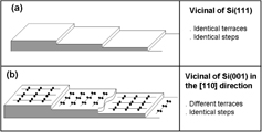
Figure 5. Sketch of vicinal surfaces.
Download figure:
Standard image High-resolution imageIn figure 5(b) we show the case of a Si(001) surface misoriented in the [110] direction. Due to the diamond structure of silicon, one terrace reconstructs with dimers parallel to the ![$[\bar 110]$](https://content.cld.iop.org/journals/2043-6262/5/1/013002/revision1/ansn488209ieqn18.gif) direction, whereas the other terrace reconstructs with dimers parallel to the [110] direction. The surface stress of the (001) terraces is thus a second rank tensor which reads
direction, whereas the other terrace reconstructs with dimers parallel to the [110] direction. The surface stress of the (001) terraces is thus a second rank tensor which reads  for one terrace and
  for the other (when written in the [110],
 ![$[\bar 110]$](https://content.cld.iop.org/journals/2043-6262/5/1/013002/revision1/ansn488209ieqn21.gif) surface axis). As a consequence, a vicinal surface misoriented in the [110] direction is characterized by a surface stress difference
surface axis). As a consequence, a vicinal surface misoriented in the [110] direction is characterized by a surface stress difference  in the direction normal to the step. It is then characterized by an elastic monopole.
3.2. Facetted surfaces
A facetted surface can be described by its mesoscopic facets (black and green facets in figure 6). Each facet can be characterized by its own surface stress. The facetted surface can thus be described as an assembly of L-apart elastic monopoles located at the facet boundaries [36, 37]. The surface stress discontinuities at the facet boundaries can be modelled by rows of elastic monopoles perpendicular to the discontinuities. At equilibrium the elastic relaxation (energy gain) induced by these surface forces balances the energy cost (β) due to the domain boundaries. It results that the period of the facetted structure is fixed by this equilibrium. In the simplest case depicted in figure 6 this period reads [36, 37]

where p = N/M is the relative coverage of one phase with respect to the other, E and ν the Young modulus and the Poisson ratio of the solid, a0 a cut-off introduced to avoid the local divergences due to the use of point forces. The surface stress components which appear in equation (13) are the surface stress components perpendicular to the edge which separates the α and β facets.

Figure 6. Elastic models for a facetted surface formed by a horizontal flat facet (label 1) and a stepped facet (label 2). The period L = Ma consists in a flat terrace followed by a step bunch. The nanoscale and Marchenko–Alerhand models are also reported. In the nanoscale model steps in the bunch are modelled by elastic dipoles (double arrows), whereas in the Marchenko–Alerhand model the bunch is considered as a microscale facet modelled by elastic monopoles (arrows) located at the facet edges.
Download figure:
Standard image High-resolution imageThe same facetted surface may also be described as an assembly of L-apart bunches of monoatomic steps characterized by elastic dipoles located at the steps edge (on the green facet). In this case the period reads [15]

where  with A⊥dip and A∥ dip the normal and tangential components of the elastic dipole.
The nanoscale and microscale models are equivalent if a0 e = a and if  , introducing the step height h, so that
  (where θ is the angle of the vicinal facet) and A⊥dip = hs1 where s1 = sxx is the surface stress component perpendicular to the step. For weak values of θ one obtains [15]

This expression is analogous to the one found by Salanon for stressed solids [38] where the steps are described by the sum of rows of dipoles and monopoles (both perpendicular to the step) and the surface stress expression is developed up to second order in θ.
Equation (7) means that since the presence of steps leads to surface stress relaxation, the surface stress is maximum for a low index surface and thus decreases with  . In contrast, the energy cost to create surface steps implies that the surface energy increases with
  . In other words, local minima (cusps) of the surface energy plot (gamma-plot) correspond to local maxima (anticusps) of the surface stress plots.
Finally note that the elastic description of the surface stress discontinuity at the step has been widely checked from grazing incidence x-ray diffraction (GIXD) [39, 40] used to measure the elastic displacement field created by steps.
In the classical Marchenko approach used to calculate the bulk deformation induced by steps, the steps are replaced by elastic forces only characterized by components normal and parallel to the average surface [36, 37]. A better description of elastic displacements and energy is obtained when taking into account the crystalline anisotropy and describing steps as 'buried dipoles', i.e. dipoles with a lever arm not necessary parallel to the surface [41].
4. Application to Si surface
4.1. Surface stress versus surface energy
In figure 7 is reported the surface free energy anisotropy obtained by Wulf inversion of the experimental equilibrium shape (T = 1373 K) [14, 42]. This method does not allow obtaining the absolute values of the free surface energies but only the relative ones. However, the absolute surface energy of the Si(111) surface at 1373 K has been obtained independently [43].

Figure 7. Surface energy (a and c) and surface stress plot (b and d) recorded for Si. On top: electronic-structure like diagram. Bottom: polar plots in the (110) plane.
Download figure:
Standard image High-resolution imageThe surface stress anisotropy of silicon is also reported in figure 7. To obtain the surface stress anisotropy plot, electromigration has been used to facet Si surfaces that belong to the equilibrium shape [15]. In this work [15] the authors have assumed that, though electromigration was the driving force for faceting, the period of faceting is still fixed by elasticity.
In this case equation (13) has to be generalized to take into account the new geometry [2] (see figure 8)
with

θ1 and θ2 the angles the facets form with the original orientation,  a geometrical factor and c an atomic unit. The surface stress components sτ i which appear in (16) are the surface stress components perpendicular to the edge τ which separates the facets α and β.

Figure 8. Sketch of a Si surface faceted by electromigration. The faceting leads to an alternation of flat and stepped facets forming the angles θ1 and θ. For α = 0 it is similar to figure 6.
Download figure:
Standard image High-resolution imageMeasuring the period of faceting thus gives access to the surface stress difference between the formed facets. In our experiments we have measured the period of faceting for various initial surface orientations. Considering a whole set of vicinal surfaces, it is thus formally possible to obtain surface stress differences between many facets and thus the whole surface stress anisotropy. More precisely in [13], the surface stress differences have been calculated by using equation (13) with a common edge energy β (since all the facets we have studied have the same common zone axis) and by calculating the bulk elastic properties (E and ν) for each crystallographic orientation. The so-obtained data lead to a set of equations whose mathematical solution should give access to the surface stress polar dependence. However, only a few of the many numerical solutions have a physical meaning. Taking into account what precedes, these solutions are the positive solutions that lead to maxima of surface stress at minima of surface energy. We find a single solution [13]. We compare in figure 7 the surface energy-plot to the surface stress. We also report their polar-plot in the (110) plane. Note that the surface stress anisotropy is much more important than the surface energy anisotropy in agreement with what we calculated for various metals in [2]. This behaviour is quite normal since it is well known that surface stress is much more sensitive to surface relaxation than surface energy.
4.2. Surface stress discontinuities
As above-mentioned, the amplitude of the elastic forces exerted by the steps on their underlying substrate can be obtained from grazing incidence x-ray diffraction (GIXD) measurements [39]. Many results have been published for metals [39–41]. For silicon, to the best or our knowledge, only the Si(7710) surface, which is a vicinal of the Si(111) 10° misoriented towards the [1–12] direction, has been studied [16]. This surface exhibits triple steps that induce an elastic field in their underlying substrate. This elastic field has been recently studied by GIXD. The strain field induced by the triple steps is well described by an elastic model in which the steps are modelled by parallel rows of buried elastic dipoles. The best fit of the experimental results is reached on the basis of the (7710) surface structure model proposed by Teys et al [44].
The value of the torque component PT of the dipole is known to be directly related to the surface stress by sh where s is the isotropic surface stress of the nominal surface and h the step height. Since the Si(7710) surface is formed by triple steps one should expect PT = 3sh where h is the height of a monoatomic step. The experimental value extracted from GIXD experiments is PT = 1.5 nN [15]. This value is not three times the value expected for a monoatomic step: PTmono = sh ≈ 0.9 θ1 nN [15]. It is quite normal since a triple step on a (7710) surface is not a simple stack of three monoatomic steps but appears to be quite defective [15, 44].
5. Conclusion
In this paper we have reviewed some results concerning the surface stress concept. We intentionally used a simplified approach to underline the fundamental differences between surface energy and surface stress. We thus avoid the use of complete theories of surface elasticity containing specific surface behaviour expressed, for instance in terms of surface elastic constants defined as surface excess of bulk elastic constants. The definition of elastic constant is an important concept [2, 45] but, up to now, their values are not available from experiments. At the same we have not developed the linearized Gurtin–Murdoch model of surface elasticity that contains an additional displacement/gradient term [11, 12, 46] nor more recent developments devoted to solid/fluids interfaces [47].
Even in the framework of our simple views, we have neglected the role of surface strain defined as the excess of bulk strain component perpendicular to the surface [2, 19, 48]. Surface strain plays a role each time a surface is submitted to a vertical external force so that its effect can be neglected in most experimental situations.
Obviously the concept of surface stress can be generalized to the concept of interfacial stress [49]. Our main conclusions are still valid, interfacial stress and interfacial energy have to be distinguished since they are of very different physical nature. For instance, recently, using the Shuttleworth relation, it has been shown that for a liquid on a soft substrate the difference between interfacial stress and interfacial energy depends on the compressibility of the superficial zone [50] so that the interfacial surface stress is equal to the interfacial energy only if the solid is incompressible in its superficial zone.
Footnotes
- 3
Note that since we only consider a surface, facing vacuum and at mechanical equilibrium, only the surface stress intervenes in the expression of the surface elastic energy. In more general situations, surface strain also plays a role [19].
- 4
This equation can be compared to the Benson definition of surface stress as a force excess at the surface:
 [31].
[31].