
Abstract
Superresolution microscopy results have sparked the idea that many membrane proteins are not randomly distributed across the plasma membrane but are instead arranged in nanoclusters. Frequently, these new results seemed to confirm older data based on biochemical and electron microscopy experiments. Recently, however, it was recognized that multiple countings of the very same fluorescently labeled protein molecule can be easily confused with true protein clusters. Various strategies have been developed, which are intended to solve the problem of discriminating true protein clusters from imaging artifacts. We believe that there is currently no perfect algorithm for this problem; instead, different approaches have different strengths and weaknesses. In this review, we discuss single molecule localization microscopy in view of its ability to detect nanoclusters of membrane proteins. To capture the different views on nanoclustering, we chose an unconventional style for this article: we placed its scientific content in the setting of a fictive conference, where five researchers from different fields discuss the problem of detecting and quantifying nanoclusters. Using this style, we feel that the different approaches common for different research areas can be well illustrated. Similarities to a short story by Raymond Carver are not unintentional.
Export citation and abstract BibTeX RIS

Original content from this work may be used under the terms of the Creative Commons Attribution 3.0 licence. Any further distribution of this work must maintain attribution to the author(s) and the title of the work, journal citation and DOI.
Prelude: talking about nanoclusters
One of my friends, Mel, was talking [1]. Mel is cell biologist (and sometimes that gives him the right). The four of us were sitting around a table during the coffee break at a conference. There were Mel and me, and his PostDoc, Teresa, and my former supervisor, Laura. Somehow we got on the subject nanoclusters. 'I always knew they'd be discovered in the end. There were these indications from the old electron microscopy data [2–4]' Mel said. 'And don't forget the biochemistry results [4, 5]', Teresa added, 'it was quite clear for many years that there was something. As you know, I always liked the idea of lipid rafts structuring the membrane [6].' 'My God, don't be silly. That's not rafts, and you know it,' Mel said, 'I don't know what you'd call it, but I sure know you wouldn't call it rafts.' Teresa raised an eye-brow, wrinkling her forehead. 'Say what you want to, but there was the idea since the nineties that membrane proteins are clustered, most likely driven by nanoscopic phase separation of lipids. Particularly in T cells, researchers found highly orchestrated assemblies of proteins during the course of signaling [7]. That's what we commonly call rafts.' 'I just wouldn't call the nanoclusters rafts' Mel said. 'What about you guys?' Mel asked Laura and me.
I knew, Laura had been critically thinking about these issues for the last couple of years. For her, 'does it make sense?' is not the right question; at least, it's not the only important one. 'It's difficult to judge all those data.' Laura is very careful about her phrasing. 'Most of the experiments were quite indirect, and I'm sort of hesitant to draw straight conclusions onto the real system. As you know, we have previously scrutinized those models by trying to understand the different experimental approaches including their pros and cons [8–10]. I'm not saying that it's all wrong, I just want to say that we don't have enough arguments for claiming that it's right.' 'Correct! I fully agree with Laura!' Mel said. 'Rafts are too small, too transient, too, too—different. You know the Lillemeier papers [3, 11–13], the Gaus papers [14–16], those are stable protein islands! They are efficient for separating things, and upon activation—click—proteins come together, and signaling is triggered'. 'But what drives the 'click'?' Laura said. 'What provides the energy to fuse the nanoclusters together? And most importantly: what are the forces that keep the nanoclusters together?'
I found a piece of paper and started a little drawing. 'Most of the results we've been discussing so far were obtained with single molecule localization microscopy (SMLM) methods. But these methods do not directly provide images. They provide localizations. A lot of dots. Here I plotted a rather random distribution of such dots. That should symbolize our protein molecules.' I put my little drawing in the middle of the table, so that everyone could see it. Mel didn't look very convinced. 'That's not random at all, what you drew. Look at those gaps, and there also appears to be clustering on various spots.'
'That's the nature of randomness' Laura said. 'C'mon, Nick, show them your computer simulations.' I pulled out my lap-top and showed them to the others (figure 1). 'Look first at panel (a), in which I plotted a random distribution of dots. I assumed here 70 molecules per μm2; this number matches the surface density of one of our favorite proteins in the lab, the T cell receptor complex [17, 18]. Also here, you find rather empty regions next to regions of high localization density.'
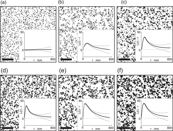
Figure 1. Comparison of various protein distributions (a)–(c) with their localization maps in an SMLM experiment (d)–(f). Insets show Ripley's K analysis of the simulated scenarios: the black curves represent the mean of 20 independent simulations, grey curves represent the standard deviation. (a) Random distribution of 70 molecules per μm2. (b) Clustered distribution of 70 molecules per μm2. 30 clusters per μm2 with a radius of 100 nm were simulated. (c) Clustered distribution of 150 molecules per μm2, with 70% of all molecules residing inside of clusters. 20 clusters per μm2 with a radius of 55 nm were simulated. (d)–(f) SMLM representation of the molecular distributions in (a)–(c). Each molecule is represented by multiple localizations. Overcounting was simulated in accordance to experimentally determined blinking statistics [19]. Localizations were distributed around the true molecular positions following a Gaussian distribution with a mean localization error of 20 nm. Scale bars: 1 μm.
Download figure:
Standard image High-resolution image'Ok, I see' Teresa said. 'That means, even if there are no mechanisms to bring molecules together, they would occasionally be together. And vice versa, if nothing separates them actively, there will occasionally be quite large distances to the nearest neighbor. But in case of additional clustering, wouldn't that be much more pronounced?'
I showed them panel (b) and (c) of figure 1. 'Here I introduced clustering, starting in panel (b) with a lot of large clusters covering almost 50% of the surface and all molecules inside the clusters. In panel (c), I assumed a few small clusters. In addition, I put some randomly distributed dots across the entire image, mimicking non-clustered molecules. In a nutshell, what you see is that there are situations, where clustering doesn't appear to be substantially different from the random case'.
We discussed these images for a while and found scenarios, in which even minor deviations from randomness may be amplified in a way that they become biologically relevant [20]. In fact, if different species of clusters co-existed where each species hosted different proteins, segregation would still be sufficiently efficient to preclude any initiation of signaling. Then Mel said 'But couldn't you easily detect even such small deviations from randomness? I mean, wouldn't the Ripley's K analysis [21, 22] pick that up?' I said 'Sure, that would be picked up. I plotted the results as insets to the according panels of figure 1.'
Laura nudged me in the side. 'Show them the other images, Nick! Those that contain the blinks!' I opened figures 1(d)–(f) on my computer. 'What you can see here are similar images as before, but I tried to mimic here a typical SMLM experiment. Each data point now represents a detected molecule—let's call that a localization, and the whole image a localization map. Can you still see the difference between randomness and clusters?' Teresa scratched her head. 'Well, to be honest, Nick, I think I can. Although I don't know exactly what you did on your computer, I see much more clustering on panel (f) than on panel (d). And that should be the clustered image, shouldn't it?' Mel nodded his head. 'I think I understand what Nick is trying to tell us here. Compare figures 1(c) and (d). If you hadn't had the comparison with the truly random case without blinking, you couldn't tell the difference. In other words: the random situation shown in figure 1(d) looks quite similar to the clustered situation shown in figure 1(c), even upon quantification via Ripley's K analysis.' 'So what did you add here, which makes figures 1(d)–(f) so much different than figures 1(a)–(c)?' Teresa said. I smiled. 'A bit of reality: a spoonful of localization errors; a pinch of diffusion; and a whole lot of blinking.'
The gong indicating the next session halted our little conversation, and the four of us headed back to the lecture room. 'It seems that the whole superresolution microscopy is useless for cell biology. Is it that what you mean?' Teresa said. As always, she was exaggerating. 'I don't think that it's useless' Laura said. 'You just have to be careful and know what you're doing.' I nodded. 'And you have to understand the mistakes—including your own.'
Single molecule localization-based superresolution microscopy—revisiting the basics
Life scientists feel the need for quantitative data as a robust basis for understanding the organization of cells at the nanoscale, and superresolution microscopy seems to provide such data. To fully capitalize on the new information, however, we have to better understand the respective imaging and analysis processes. In this chapter, we provide a brief introduction to SMLM techniques, accenting the major differences to standard microscopy.
Commonly, fluorescence imaging via high-quality microscopes is considered to be linear and shift-invariant. With linearity, we mean that if two objects  and
and  are imaged to
  and
and  then their weighted sum
  is imaged to
  Linearity depends on the quality of the detector and requires the absence of fluorescence quenching or shading within the object. Shift-invariance means that the image of a point object is the same in the whole field of view. No imaging system is perfectly shift-invariant, yet for many high-quality research systems the condition is met to an excellent approximation.
If linearity and shift-invariance are fulfilled, the overall intensity distribution of an image is the convolution of the (continuous) spatial distribution of emitters,  with the point spread function of the imaging device,
  [23]:
[23]:
In practice, samples consist of individual emitters located at position  We can thus write for the discrete spatial emitter distribution function
where N denotes the total number of emitters and  the Dirac delta function. In principle, different emitter molecules may show different (time-averaged) brightness
  for example due to fixed or constrained orientation of their transition dipole moments, the presence of nearby quenchers, or simply stochastic fluctuations of the photon number detected from each molecule [24]. We can account for this in the spatial emission distribution
The total intensity distribution then simplifies to
Uncovering the emitter distribution  (or
(or  ) would be microscopists' ultimate goal, and various algorithms have been proposed to deconvolve equation (1) or equation (2) in order to obtain a good estimate of
  [25]. The problem, however, becomes mathematically ill-posed, whenever high spatial frequencies in
  shall be uncovered, leading to the classical diffraction-limit in microscopy. In that case, the point spread functions of the individual emitters overlap strongly, and marginal fluctuations of the recorded signals on the camera have a decisive impact on the obtained shape of
The general idea behind SMLM is the consideration of additional parameters, which allows for singling out a subset of dye molecules. A single image then contains only signals from a small fraction of all dye molecules, which are likely separated far enough to avoid any signal overlap. By tuning the additional parameter deliberately or stochastically and recording multiple images, one can ultimately collect signals from all dye molecules within the sample.
To our knowledge, the first realization of this idea was demonstrated in a study by van Oijen and colleagues, in which the narrow and distinct lines in the excitation spectrum of fluorophores at low temperature were used to single out individual dye molecules within a sample of rather high densities of dyes [26]. The distribution function of signals then becomes
where  describes the probability that the molecule i will be detected at the excitation frequency
  Ideally,
  is essentially zero over the whole spectral region except for a single narrow spike, where the particular molecule is at resonance with the excitation laser. Thereby, the resulting signal density on each image becomes low enough to preclude overlapping point spread functions. The deconvolution problem hence gets massively simplified to the problem of finding the emitter positions of well-separated signals. Such problems are well known from the field of single particle tracking [27]; particularly, the center position of a noise-limited signal distribution can be determined with accuracy far below its actual width [28], thereby paving the way for circumventing the resolution limit of light microscopy.
The observation of blinking [29] or photoswitchable fluorophores [30–32] gave rise to new and simpler concepts, which do not depend on observations at low temperatures: instead, the emissive state of dye molecules can be switched stochastically in time between a dark state and an active state [33–35] (figure 2). In that case, we can rewrite the spatial emitter distribution function as
where  is a Boolean function describing time-dependent fluctuations between dark and active state. Here, time is measured in units of the frame number within the respective image sequence. Note that for our formalism, the physical principle behind the blinking is not important. SMLM variants include points accumulation for imaging in nanoscale topography (PAINT) [36–38], which utilizes the transient binding of a fluorescently labeled probe to its target, and binding-activated localization microscopy (BALM) [39], where the binding of the probe additionally increases its brightness.

Figure 2. Generation of localization maps in SMLM. Top to bottom: Labeled protein molecules are sequentially switched between fluorescent (indicated by color) and non-fluorescent dark states. Localization maps contain the positions  of all observed single molecule signals. The determined localization differs from the true position of the protein,
  due to fitting errors
  and localization bias,
  In addition, residual diffusion of fixed molecules can add to the spread of the recorded localization (indicated for the protein labelled with the red color at t = 2).
Download figure:
Standard image High-resolution imageIdeally, each emitter is imaged only once. In this case,  would be zero except for a single spike with length of one image, where the fluorophore is active. In practice, however, emissive states of a single dye molecule with varying length and interjacent dark periods may be spread over the whole imaging sequence [40, 41], leading to repeated detection of the same molecule (i.e. overcounting). In contrast, undercounting arises e.g. from incomplete labeling due to non-saturating antibody concentrations or inaccessible epitopes in immunohistochemistry, from the presence of non-activatable dyes conjugated to the antibody, or from the termination of the imaging sequence before activating all fluorophores. The parameter
  can be used to account for both overcounting and undercounting: overcounting can be modelled by multiple spikes in
  undercounting by setting
  for all times
It was recognized early in the field, that isotropic point emitters can be localized to a precision much below the diffraction limit of optical microscopy [28]. Thompson et al provided a first comprehensive analysis of the dependencies of localization errors on parameters like signal intensity, background, and pixel width [42]. Under ideal conditions (i.e. high signal brightness and low background noise), localization precision of 1 nm [43] and below [44] were reported. Thompson et al, however, also realized in their paper that the obtained equations underestimate the true errors by approximately 30%. Later, localization algorithms were developed, which achieve localization precision at the Cramer–Rao bound [45, 46]. See [47] for a review on various issues related to single fluorophore localization.
To obtain an SMLM image, researchers construct localization maps, which are visualized using one of a variety of rendering algorithms [48–50]. Typically, tens of thousands of images are recorded in order to reconstruct a single localization map. One common visualization method is Gaussian rendering. It assumes that localization errors are unbiased and can be reasonably well described by a normal distribution, with a standard deviation given by the estimated localization errors  In this way, however, blurring due to localization errors is slightly overestimated: if we assume a true localization error
  the resulting distribution of localizations is a convolution of a Gaussian of
  with a second Gaussian of
  yielding a total Gaussian of
  [51]. Some researchers instead make use of averaged shifted histograms, which provide a valid and computationally efficient estimator of the probability distribution of localizations [52].
In practice, however, the assumption of an unbiased error distribution may be not correct. First, antibodies (and secondary antibodies) are frequently used for labeling the protein of interest, thereby separating the observed dye molecule from the labeled biomolecule. Given the size of an antibody of ∼10–15 nm [53], standard labeling tools may well displace the observed localizations by up to 30 nm from the protein of interest. Secondly, the transition dipole radiates anisotropically, which generally results in deviations from a centrosymmetric Gaussian-shaped point spread function. The effect becomes dramatic in case of fixed dipoles [54], or aberrated or defocused images [55]; even for rotating dipoles, shifts of the Gaussians do not completely average out in case of constrained rotation and slightly defocused imaging conditions [56]. This will lead to biases in the determined x/y positions, if centrosymmetric functions were used for localizing the molecules. In addition, non shift-invariant imaging conditions, particularly at the edges of the field of view, may contribute to biased localization errors.
Taken together, we can expect biased error distributions centered at a position  The reconstructed superresolution image is hence described by
Important for SMLM is to ensure that the structures of interest do not move during the recording process; ideally, all observed molecules are perfectly immobilized. The common strategy towards this goal is the usage of chemical fixatives such as paraformaldehyde or glutaraldehyde, which extensively cross-link cellular proteins [57]. In practice, however, chemical fixation leaves a substantial fraction of molecules rather mobile, which shows residual mobility with a diffusion constant of up to Di = 0.01 μm2 s−1 [58]. Hence, the position  and the bias
  become a function of time:
The overall goal would be to reconstruct the starting positions of all molecules,  from the obtained image
  Although equation (3) contains essentially all relevant parameters it is not very helpful, since the values of virtually all parameters are unknown:
- Although we know precisely the time of appearance for each single localization, we cannot assign it unambiguously to a certain molecule i. Hence,
 is unknown.
 - In consequence, also the number of molecules, is unknown.
- The positions are unknown, particularly for the time periods where the molecules are invisible.
- The bias is likely different for different molecules, for example due to different orientational constraints of the labeling antibody or the attached fluorophore. It may also vary with time, if the residual diffusion changes the orientation of the attached antibody.


Only the localization errors  can be estimated fairly well from the brightness of the signal and the background fluctuations [45].
We can improve the situation by minimizing some sources of error; for example, better fixation procedures may reduce residual diffusion, and also the size of the label can be reduced by using direct labeling instead of indirect approaches. In addition, control experiments can be performed to estimate the unknown parameters. Still, we are far from solving equation (3) for 
Even more so, superresolution microscopy deals with random processes such as the stochastic switching of molecules from inactive to active states, the localization errors, and the residual Brownian diffusion of the labeled molecules. It may hence be more appropriate to view the problem as a stochastic process. The likelihood of detecting a single localization of molecule  within the interval
 ![$[{\vec{r}}_{loc},\,{\vec{r}}_{loc}+d{\vec{r}}_{loc}]$](https://content.cld.iop.org/journals/2050-6120/7/1/013001/revision2/mafaaed0fieqn47.gif) in the frame number
in the frame number  is then given by
It can be calculated from the probability density function for localizing a molecule at position  given that it was actually located at
and the probability density function for Brownian motion (assumed here in 2D) of a particle starting at position  at time
  and moving with
  [59]
[59]
![${p}_{diffusion}({\vec{r}}_{i}| {\vec{r}}_{i,0})d{\vec{r}}_{i}=\displaystyle \frac{1}{4\pi {D}_{i}t}\cdot \exp \left[-\displaystyle \frac{{({\vec{r}}_{i}-{\vec{r}}_{i,0})}^{2}}{4{D}_{i}t}\right]d{\vec{r}}_{i}$](https://content.cld.iop.org/journals/2050-6120/7/1/013001/revision2/mafaaed0fieqn54.gif) From this, we can estimate the two-dimensional probability distribution of localizations in the final superresolution image
From this, we can estimate the two-dimensional probability distribution of localizations in the final superresolution image
Here,  denotes the average number of localizations detected from molecule
  Equation (4) has the advantage over equation (3) that it captures the probability of a localization map, which—in principle—should be close to the averaged shifted histograms determined experimentally.
A closer look onto the equation (4), however, reveals also here several limitations:
- In our derivation, we have assumed uncorrelated single molecule parameters in time. This is, however, in general not fulfilled. For example, the diffusion process leads to correlated appearances along the trajectories of the individual molecules. In consequence, a realization of a superresolution experiment with diffusion yields extended, slightly asymmetric localization clusters [60] (figure 3). Also localization biases likely persist over time. Finally, repeated detections of single molecules are not uniformly distributed across the image sequence, but usually accumulate within a few hundred frames [61].
- Also data from different molecules in the same sample could be correlated. For example, secondary antibody labeling makes microtubule larger than they really are [62] due to correlated localization bias. In addition, background noise and overlapping signals in dense regions of the sample easily lead to localization bias [63, 64].
- If molecules are part of a larger cellular structure, fixation connects them. In consequence, their joint residual diffusion correlates.
- Finally, equation (4) only provides a solution for the probability of obtaining a localization map, but not for the probability of the starting positions


First interlude
'That was a tough one' Mel said. 'Nick, your background is physics, could you please translate that to us?' The four of us had left the session to get some fresh air. 'I'm not exactly sure what this guy wanted to tell us. It was quite heavy on the formulas. I think, his aim was to put those arguments I raised before into mathematical equations. But he didn't get very far, the formulas just showed the problems, but didn't provide solutions. A lot of unknowns at the end.'

Figure 3. The effects of residual diffusion on localization maps. Clustered distribution of 70 molecules per μm2. 10 clusters per μm2 with a radius of 30 nm were simulated. Each molecule is represented by multiple localizations. Overcounting was simulated in accordance to experimentally determined blinking statistics [19]. Localizations were displaced from the true molecular positions with a mean localization error of 20 nm following a Gaussian distribution. (a) Ideal situation of completely fixed molecules. (b) Molecular clusters exhibit a residual diffusion with D = 10−4 μm2 s−1. An image sequence of 103 frames at a framerate of 100 Hz was simulated. Scale bars: 1 μm.
Download figure:
Standard image High-resolution imageLaura pulled out her notes. 'These are my take-home messages:
- Number of molecules: it is not equal to the number of localizations, could be more, could be less.
- Localization errors: the determined localizations do not reflect the true molecule's position. Errors follow a normal distribution; its sigma-width may vary between molecules, and it may not be centered at the protein's position.
- Residual diffusion: Molecules are not completely immobilized after fixation. Some move faster, others hardly move at all.
- Correlations: the math becomes tricky due to correlations between different molecules.'
Teresa fiddled with her mobile phone and said: 'In the next session, there will be a talk on fluorophore blinking. Shall we have a look? I mean, if one understands blinking, probably the unknowns of this guy become knowns?'
Photoactivation and photoswitching in SMLM
SMLM is based on switching fluorescent probes between two states: one bright state, which is detectable by the optical system ('on'), and one state which is dark or at least invisible for the optical system ('off'). Experimentally, this is realized by using photoactivatable, photoconvertible or photoswitchable fluorescent proteins (FPs) in photoactivated localization microscopy (PALM), and by chemically induced blinking of organic fluorescent dyes in (direct) stochastic optical reconstruction microcopy ((d)STORM). The switching ideally occurs only between these two states and is controlled by the operator. This would allow for precise tuning of the number of molecules visible on each single frame—a necessity for keeping the density of visible molecules low enough for the unambiguous detection of single molecules—and the number of times a molecule is detected throughout the recorded image sequence.
However, not a single out of a hundred described fluorescent molecules used for SMLM sticks to this ideal scenario: the existence of multiple dark states and the process of photobleaching challenges this simplified view. The particular physico-chemical mechanism for switching depends on the type of molecule and differs fundamentally between FPs and organic dyes. In the following we discuss molecular mechanisms responsible for the transition between different states. We restrict ourselves here to new, monomeric, and bright representatives of FPs (for a comprehensive review on FPs available for SMLM see [65–67]) as well as some prominent examples of organic dyes (for a more detailed review of organic dyes used for superresolution see [68, 69]).
Photoactivatable and photoswitchable fluorescent proteins
Stochastic switching between 'on' and 'off' states of GFP and YFP was first described by the Moerner group more than two decades ago [29]. The first FP which could be controllably switched by irradiation with UV-light was a genetically modified version of GFP termed photoactivatable GFP (PA-GFP) [30]. Analysis of the x-ray structure revealed the mode of action: UV-irradiation causes the decarboxylation of glutamine at position 222 that shifts the chromophore from the dark, neutral trans ('off') to the bright, anionic cis conformation ('on') [70], concomitant with a ∼100-fold increase in fluorescence. The anionic state of the chromophore now forms a pi-conjugated electron system, which gives rise to the fluorescent property of the FP. Importantly, the off-on switching reaction is unidirectional; such proteins are hence named (irreversibly) photoactivatable (PA)-FPs (table 1). Another prominent representative of this group is PAmCherry, which sticks out due to its superior 5000-fold fluorescence enhancement upon UV light irradiation [71]. For all PA-FPs, the switching from 'off' to 'on' is induced by UV-light irradiation [65]. A switch back to the 'off' state is not possible. Figure 4 (left panel) shows a generalized state model, which displays these interconversions between states. For PA-FPs, the 'on' rate, kon, depends on the UV light intensity, whereas koff equals zero due to the unidirectionality of conversion. In the simplest model for ideal PA-FPs, the protein finally transitions to a 'bleach' state due to light-dependent photodamage.
Table 1. Groups of fluorescent proteins used in SMLM.
| Group | 'Off'-state | 'On'-state | kon | koff | Examples |
|---|---|---|---|---|---|
| Irreversibly photoactivatable | dark | fluorescent | Light-dependent | 0 | PA-GFP, PAmCherry |
| Irreversibly photoswitchable | fluorescent | fluorescent | Light-dependent | 0 | PS-CFP, mEos, Dendra2, mKikGR |
| Reversibly photoswitchable | dark or fluorescent | fluorescent | Light-dependent | Light-dependent | Dronpa, rsEGFP |
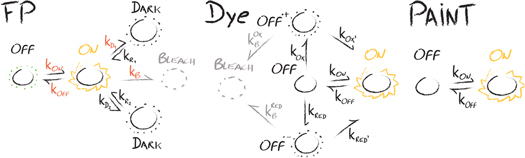
Figure 4. Models of interconversion of states for fluorescent proteins (left), organic dye molecules (center), and in PAINT [72] (right). (FP) For photoactivatable and photoconvertible FPs the transition from the thermodynamically stable 'off' state is triggered by light irradiation and is unidirectional, i.e. koff = 0. Reversibly photoactivatable or photoswitchable FPs can be repeatedly toggled between the 'on' and the 'off' state. The presence of short and long lived 'dark' states cause unwanted blinking of FPs. Transition into the 'bleach' state is caused by permanent photodamage. Light-induced transitions are shown in red. (Dye) Intersystem crossing causes the population of the 'off' state in organic fluorophores. Upon presence of a reduction/oxidation system (ROXS), the 'off' state is rapidly depleted by electron transfer either through oxidation by forming a radical cation (OFF.+) or through reduction by forming a radical anion (OFF.-). The two possible radicals are rapidly recovered to the 'on' state due to the presence of ROXS, hence preventing the population of the 'bleach' state [73]. (PAINT [72]) In the 'on' state, the dye-labeled imager strand is bound to the docking strand on the molecule of interest. The respective rate, kon, can be tuned by adjusting the concentration of the imager strand. In the 'off' state no labeled strand is present. The 'off' rate, koff, depends strongly on the overlapping length of imager and docking strands.
Download figure:
Standard image High-resolution imageThe same state model holds for the group of irreversibly photoswitchable FPs (table 1), which shift the emission wavelength upon irradiation with ∼400 nm light. Here, the 'off' state is not dark, but a fluorescent state that is blue-shifted compared to the 'on' state. For PS-CFP [74] and the improved version, PS-CFP2 [75], a decarboxylation similar to PA-GFP is responsible for switching the protein from a cyan to a green fluorescent state at a contrast ratio of ∼2000 [75]. Other examples of irreversibly photoswitchable FPs include mEos3.2 [76], Dendra2 [75] and mKikGR [77], which are converted upon cleavage of the peptide backbone of a histidine. This creates an elongated pi-conjugated electron system of the chromophore and causes the red-shift of the fluorescence emission.
Reversibly photoactivatable or photoswitchable FPs define a third group of protein labels (table 1) used for superresolution microscopy, which can be repeatedly toggled between the 'on' and the 'off' state. The photoswitching mechanism involves a change of the chromophore's isomerization and protonation state as well as a rearrangement of amino acids in its close environment [67]. In contrast to PA-FPs, the fluorescent cis configuration is the energetically favorable state for reversibly photoactivatable or photoswitchable FPs. Without illumination, relaxation to this state proceeds on time scales of minutes to hours and can be actively triggered by light irradiation. A well characterized representative is Dronpa, which can be switched to the dark 'off' state with 490 nm light and back to the bright 'on' state upon UV irradiation [78]. If bleaching is neglected, both rates - kon and koff - depend on the laser intensity at the respective wavelength. After ∼100 on-off switching cycles, 75% of Dronpa molecules are still active, i.e. unaffected by photobleaching [78]). Recently developed proteins are even capable to survive several thousands of switching cycles before terminal photobleaching, and they also show faster switching rates. It is worth noting, that in contrast to all other reversibly photoactivatable or photoswitchable FPs, photoswitching of Dreiklang is based on a reversible hydration/dehydration reaction rather than a chromophore isomerization. Additionally, photoswitching is de-coupled from fluorescence excitation: while for other PS-FPs the fluorescence excitation of the molecule in the 'on' state causes switching back to the 'off' state, this does not happen in Dreiklang. Only illumination with light at a shorter wavelength than the excitation wavelength triggers the conversion to the 'off' state. This allows for precise control of the duration of each photoswitching cycle. For Dreiklang, the rates kon and koff depend on the intensity of the switching wavelengths, which are both shorter than the one used for excitation for fluorescence detection [79].
Recently, more sophisticated molecules were engineered which combine features of both, reversibly and irreversibly photoactivatable FPs. IrisFP [80] can be irreversibly photoconverted from a green to a red fluorescence form upon UV irradiation. Both forms can undergo cis-trans isomerization and thus can be switched between a dark and the respective fluorescent state. This enabled entirely new experimental approaches, like pulse-chase imaging combined with SMLM [81].
All rates described so far can in principle be determined and the optimal FP can be chosen based on the requirements for the SMLM experiment. However, in addition to light-controlled photoswitching between 'on' and 'off' states, also unintended stochastic transitions between the states occur, giving rise to blinking. These include the presence of long-lived 'dark' states, which were described e.g. for mEos2 [40, 61] and PA-GFP [82], as well as short-lived 'dark' states, which were detected for various FPs [83]. A detailed analysis of mEos2 and Dendra2 blinking yielded a kinetic model [84], which accounted for both a slow and a fast recovery rate back from the 'dark' state, kr1 and kr2, and a single rate from the 'on' to the 'dark' state, kd = kd1 = kd2 (see figure 4, left). By studying the flickering of Dendra2 using fluorescence correlation spectroscopy (FCS), a recent study revealed that the two 'dark' states can be populated from both, the green ('off') and red fluorescence ('on') state [41]. By varying the pH the researchers concluded, that the rate for entering the first 'dark' state, kd1, depends on the light-dose of fluorescence excitation. The subsequent chromophore protonation arises from a proton exchange between the chromophore hydroxyl group and one or more internal proton binding sites [41]. The rate for entering the second 'dark' state, kd2, depends on the availability of free protons in the bulk solution (see figure 4, left).
Stochastic photo-blinking of organic dyes
Similar to the photo-induced activation or switching of FPs as the basic concept for PALM, photo-blinking of organic rhodamine and cyanine dyes is the prerequisite for SMLM via (d)STORM [33, 85]. Overall, at least three modes of blinking have been described [29, 73, 86, 87] (figure 4, center panel). First, the spontaneously occurring inter-system crossing from the excited singlet state S1 ('on') to a dark triplet state T1 ('off') blocks the new excitation, thus keeping the fluorophore dark. T1 has a lifetime of several microseconds, after which the fluorophore relaxes back to the ground state S0 and can be excited again. Second, by adding a reduction/oxidation buffer system (ROXS), the triplet state T1 gets rapidly quenched by either reduction or oxidation of the fluorophore (OFF.−/OFF.+), resulting in non-fluorescent radical ion species. These dark states can be stabilized for up to seconds; the lifetime of this radical ion can be controlled efficiently by adjusting the concentrations of the reducing and oxidizing agents [73], thus regulating the time until the fluorophore relaxes back to its original ground state S0. Bleaching can occur from both of these dark states. Third, photochromic blinking is described by the reversible photoinduced transition between two chemical species of a fluorophore [29, 87] other than oxidation or reduction.
The aim in STORM is to reduce fast triplet blinking, while introducing prolonged dark states due to redox or photochromic blinking. The first realization of STORM was described using an oxygen scavenging buffer system made of glucose, glucose oxidase and catalase to quench the triplet state, and the addition of β-mercaptoethanol or β-mercaptoethylamine as reducing agent [33]. One proposed mechanism is, that upon excitation, the cyanine dye Cy5 undergoes a photochromic change by reacting with thiol groups [85, 88]. This transition could be reversed by either excitation with shorter wavelengths (direct STORM [69, 85]), or by addition of an additional activator dye, Cy3 [33]. Buffers consisting of different oxygen scavenging systems supplemented with reducing and/or oxidizing agents have been reported and yielded different results for various dyes [68]. The above mentioned mechanism, however, is questioned by the high activation energy of C–S bonds, created by reaction with thiols, as well as by the absence of absorption in the visible spectrum for these bonds. Additionally, the generation of radical species upon oxidation and reduction of cyanine dyes was reported, representing an alternative mechanism for blinking [89].
A different way to facilitate blinking of fluorophores is PAINT [36]. In a nutshell, in PAINT blinking is not induced by the chemical surrounding of organic dyes, but solely governed by the binding kinetics between the fluorescent probe and a molecule of interest. Each bound and hence immobilized probe can then be localized with high precision, while the signal of unbound probes vanishes in the background. The contrast between bound and unbound molecules can further be enhanced by using fluorogenic probes [39]. Such probes feature increased brightness upon binding to their target, facilitated e.g. by the target's environment. Hence, probes used in PAINT range from membrane probes, such as NileRed [36], to more generic ones, such as DNA-modified probes with complementary DNA strands being present on the organic dyes [72]. For the latter a simple two state model similar to PS-FPs can be assumed (figure 4, right panel), with kon and koff being dependent on the probe concentration and length of the overlapping DNA strands, respectively.
Second interlude
'I like the physical chemistry talks!' Laura said, after we left the room. 'Everything's so clear! You can calculate the rates, adjust the redox conditions. That's scientifically sound!' Teresa teased: 'Sure! You can calculate precisely that these compounds will never be good for anything! And as we just heard, even the physical chemists don't always concur!' Mel nodded his head. 'I sort of agree with Teresa.' He pulled a piece of paper out of his bag. 'Look, I've tried to summarize the key figures of the last presentation. In figure 4 you see the 'on'-'off' transitions that may occur in fluorescent proteins. That's a complete mess! Sure, you can determine all the rates: but in practice, these foolish things blink on all possible time scales, and you'll never be sure whether a molecule that you have already imaged suddenly decides to reappear, or a new one pops up for the very first time!'
I smiled. 'And still those little things remain - that bring me happiness or pain. But let's see whether things are really that bad. Fluorescent proteins could be difficult, I agree. But look at figure 4(b), where you plotted the transitions for the organic dyes. That's not bad at all. You can get dyes with well-defined on-off kinetics. I admit, we still have the problem of stochastics—some molecules will blink more often than others. But we know the statistics, and they are identical for all molecules of the same type in the sample.' Mel added another drawing. 'This lady spoke too fast for me, I had no time for the PAINT method. I added it now as panel (c). That indeed looks much better. There, you have essentially only one pathway for the off-on transitions.'
Teresa didn't appear too convinced. 'You guys completely forget about the complexity of biological systems. You argue that organic dyes blink, as if they were in a perfectly adjusted and pure environment. But in fact, they aren't. There may be locally altered redox, quenching, or protonation conditions. Couldn't it be, that the environment varies from one molecule to the next ? And what about linking your perfect dye to the protein of interest?' By hitting these valid points, Teresa efficiently switched off Mel and me. Only Laura remained active. 'Well, most people would rely on immunohistochemistry; they'd label with a dye-conjugated antibody, or use a non-fluorescent primary and a dye-conjugated secondary antibody. That makes things worse again: the on-off transitions now further depend on the number of dyes linked to a specific protein molecule. That can easily lead to a labeling ratio of ten or even more dyes per protein.' Teresa got going now. 'Even worse: you don't know anything about the statistics of the dye to protein ratio. Likely, the bound fluorophore affects the binding of the antibody. In other words: it may be that only the weakly labeled antibodies can bind their target protein [90].' Laura nodded her head. 'Or the other way 'round. One simply doesn't know. So back to FP's? At least, the degree of labeling would be clear then.' 'Not really', Teresa lectured. 'Up to now, we just considered too many counts per molecule. But it could also happen that we have too few!' The three of us didn't understand. 'Not every FP is in fact matured [91], not every protein is labeled with an antibody [92], not every oligonucleotide is accessible to its label strand in DNA PAINT.'
The gong stopped Teresa. The four of us decided to move on to a symposium session on methods to detect protein clusters in membranes. 'Let's see what those guys will tell us' Mel said. 'I'm not so convinced about that stuff anymore.'
Methods for detecting nanoclusters
SMLM has been providing fascinating new insights into the molecular organization of biological samples. It must be borne in mind though that the methods only yield point patterns of localizations. Appropriate analysis is necessary to conclude from localization maps onto the spatial distribution of molecules at the cellular plasma membrane. Currently, however, a number of different analysis approaches are being used without a clear consensus how to disentangle true molecular clustering from localization clusters of blinking fluorophores. In the following, we give an overview of methods used to analyze SMLM images, particularly with respect to their ability to detect and quantify nanoclusters of plasma membrane components.
The human brain is skewed to identify patterns, and even randomness may appear non-random. Researchers thus rely on computational algorithms to identify and quantify non-random molecular distributions. In the following, we discriminate three classes of approaches: the first class analyzes 2D point patterns with respect to spatial randomness (figure 5), the second class compares point patterns of the samples with separately recorded standards (figure 6), the third class can be seen as a combination of the first two classes (figure 7).
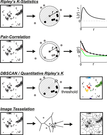
Figure 5. Schematic representation of common algorithms to analyze spatial randomness. Ripley's K–Statistics count the number of neighboring localizations (shown in black) inside circles with increasing radius r around each point. Sample data (black line) are compared to spatial randomness (grey line). Pair-Correlation based algorithms count the number of points (shown in black) inside a ring with increasing radius r around each point. The resulting correlation function (black line) is fitted with a model for overcounting (green line) and real clustering (red line). DBSCAN and Quantitative Ripley's K both rely on counting the number of neighboring localizations (shown in black) inside circles of fixed radius R around each point. Application of a threshold ultimately leads to identification of individual clusters. Image Tessellation algorithms divide the image in tiles based on the point coordinates or densities. Sketch shows a Voronoi-tessellation.
Download figure:
Standard image High-resolution image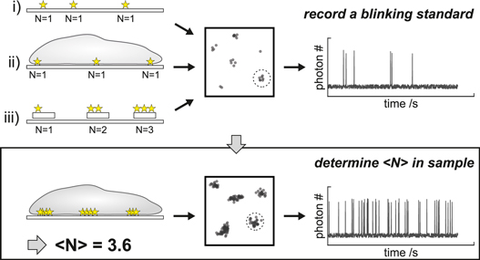
Figure 6. Schematic representation of molecular counting via a blinking standard. (top) Blinking standards can be recorded by sparsely distributing fluorescent labels on glass (i), by sparse labeling of the sample structure (ii) or by using nanoplatforms with a known labeling stoichiometry (iii). The blinking statistics of individual (i and ii) or known numbers of fluorescent labels (iii) can be determined for spatially well separated fluorescent labels. (bottom) Using such blinking standards allows to quantify the number of labels per molecular complex in a biological sample.
Download figure:
Standard image High-resolution image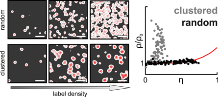
Figure 7. Schematic representation of label titration microscopy. (left) Variation of label density leads to characteristic changes in the localization maps (here illustrated on simulated data); image sizes 2 × 2 μm. (right) The normalized density of localizations inside of clusters  are plotted as a function of the relative area covered by clusters
  Deviation from the reference curve for random distributions (red line) allows for discrimination of clustered (gray) from random distributions (black).
Download figure:
Standard image High-resolution imageAnalysis based on spatial randomness
Ripley's K function [22] is a prominent member of the first class. It counts the number of points within a distance r of another point. Typically, researchers use its linearized variant, the so-called H-function  A constant value of
  is indicative of a random point distribution, whereas clustered point distributions yield a pronounced maximum approximately at the cluster radius [21]. Often, the amplitude and position of this maximum are used to make comparative statements about the degree of clustering and to estimate the average size of clusters, respectively. Notably, however, the maximum position is not only affected by the cluster size but also by their mutual distance, which impairs unambiguous quantitative conclusions [21]. Further, Ripley's K analysis captures global clustering behavior but per se does not identify individual clusters. It can be seen as an ensemble approach, which does not draw conclusions on the individual clusters. To overcome this limitation, Owen et al [93] implemented a quantitative variant, previously put forward by Getis and Franklin [94], that assigns a linearized clustering score at a user-defined radius
  to each localization. The resulting weighted point patterns are then fitted with a 2D polynomial, yielding density-dependent heat maps. Application of a threshold
  allows for creating binary cluster masks, which can be used for quantitative analysis of individual clusters to obtain information e.g. on the number of clusters, or their size distributions.
Along similar lines, density-based spatial clustering of applications with noise (DBSCAN) [95] is often used to discriminate clustered from non-clustered localizations. DBSCAN calculates for each point the number of neighboring points within a fixed radius  This number is now used for a local analysis: if it is larger than a predefined threshold
  the point is assigned to a cluster, otherwise it is not. Collectively, the application of DBSCAN to 2D point-distributions is straightforward and allows to robustly identify and characterize arbitrarily shaped clusters. Finally, also image tessellation [96, 97] has been used to determine the spatial randomness.
A drawback of both the quantitative variant of Ripley's K analysis and of DBSCAN is their strong dependence on the key parameters  and
and  To address this issue, Rubin-Delanchy et al proposed Bayesian cluster identification [98]. Here, a probability algorithm searches through a large number of possible combinations of the two parameters, generating thousands of cluster proposals, and ultimately assigns a model-based probability to each combination. The parameters with the highest probability score are then used for display and analysis of the data.
Algorithms based on the detection of spatial non-randomness are well-suited to reliably detect and quantify clustering of 2D point-distributions. They cannot, however, discriminate between true protein clustering and localization clusters arising from the repeated detection of the same dye molecules. The problem becomes apparent when localizations of a typical SMLM experiment are color-coded according to their time of appearance (figure 8): localizations that belong to the same cluster also turn out to appear highly correlated in time, which is indicative of multiple observations or 'bursts' of a single dye molecule. In their seminal work, Annibale et al proposed an empirical solution to this problem, which aims at combining multiple localizations from a single dye molecule to a single event [40, 99]. Localizations presumably originating from the same dye molecule are selected based on their spatial and temporal proximity. In this approach, however, the user-defined thresholds have a rather strong influence on the results, making it difficult to unambiguously identify protein clusters.
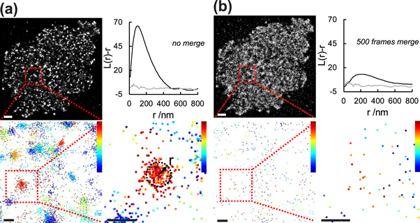
Figure 8. Time-correlated appearance of localizations in SMLM. Data are shown before (a) and after (b) processing to compensate for multiple observations of single fluorophores within a radius of 35 nm and over 500 frames, using the method proposed by Annibale et al [99]. (top) PALM localization maps of a fixed resting T cell (JCaM1.6), stably expressing Lck-mEos3.2; Ripley's K analysis of the cell (black curve) compared to a simulated random point distribution without blinking (gray curve). Scale bar: 1 μm. (bottom) Zooms of indicated areas (red boxes); localizations are color-coded according to the frame of appearance (range: frame 1–5 000); for merging, localizations are combined within a user defined radius r, corresponding to the localization error. Experiments were performed as described in Baumgart et al [100]. Scale bars: 100 nm.
Download figure:
Standard image High-resolution image
To become independent of such corrections, Sengupta et al [82] suggested to use pair correlation analysis (PCA) for detecting clustering. PCA quantifies the increased probability of finding a neighboring point at distance  compared to uniform distributions. A PCA curve ideally consists of two more-or-less well separated components, corresponding to true extended clusters and multiple observations of a single dye molecule. However, incomplete chemical fixation [101] may result in residual fluorophore diffusion, thereby increasing the size of blinking-induced localization clusters, which then are difficult to disentangle from true protein clusters. Additionally, the method struggles with the detection of clusters that are not significantly larger than the spread of localizations obtained from a single fluorophore.
Analysis based on independent recordings of single molecule blinking standards
A different scientific problem is the detection and quantification of multimolecular complexes. Examples include the nuclear pore complex [102] or clathrin-coated pits [100, 103]. While such molecular complexes can be reliably resolved by SMLM, the repeated detection of individual labels makes the counting of the involved proteins challenging. A possible workaround is the independent determination of the blinking statistics of a single label molecule, which can be compared to the data obtained on the biological sample. Generally, it is important to record the single molecule standards under identical conditions as the actual biological sample. Particularly, experiments performed under limiting dilution on the cellular system are preferential over the recording of standards unspecifically adsorbed to the glass surface, for the following reasons: (i) photophysics may vary for a cell-bound dye-labeled antibody and the same antibody adsorbed to a glass surface; (ii) glass-adsorbed labels may not be identical to cell-surface bound labels. For antibodies, for example, it is known that binding specificity decreases with increasing degree of labeling, making cell-bound antibodies preferentially labeled at lower stoichiometry [90]. (iii) free dye may contaminate the signal from the glass surface.
Interesting experimental implementations of this concept include Ehmann et al [104], who determined the stoichiometry of protein clusters based on the titration of fluorescently labeled primary and secondary antibodies. Nieuwenhuizen et al [105] employ the buildup of spatial image correlation during acquisition to derive a detailed model of fluorophore activation, bleaching and labeling stoichiometry, which allows for quantitative analysis of single molecule distributions. Alternatively, DNA origami were used as synthetic standards, which allowed for deliberate variation of the amount of colocalized fluorescently labeled proteins [106]. For FPs, tandem constructs were used as calibration standard [107].
Frequently, researchers assume three state kinetic models of fluorophore photophysics [84, 105, 108]. Here, a fluorophore can be either permanently bleached or change to a reversible dark state after its activation (see also figure 4). Such models are then used to fit the distribution of localizations per molecular complex, yielding an ensemble estimation of the number of molecules per oligomer. In general, however, fluorophores may exhibit additional fluorescent or dark states making the underlying photophysics more complicated. Taking this into account, Hummer et al [109] proposed a method to count molecules, where the functional form of the blinking statistics becomes independent of the underlying photophysics. These approaches perform best in sparse to medium protein densities [1–25 molecules/μm2). At too high densities, however, random co-localizations of the molecule of interest will lead to the overlap of individual localization clusters, thus making a reliable counting of blinks per complex difficult.
Combination of the two approaches
As a combination of the two concepts, Baumgart et al developed a method to assess the randomness of protein distributions, based on implicit recording of molecular standards [100]. The approach does not directly count the number of localizations per fluorescent label but makes use of the characteristic changes in the localization maps upon variation of label density. These changes are quantified by standard cluster analysis tools and plotted as  vs
vs  where
where  denotes the density of localizations inside the clusters, and
  the relative area covered by localization clusters (figure 7).
While  hardly depends on
  in case of a random distribution, clusters yield a characteristic increase of
  over
over  which allows for robustly discriminating between the two scenarios independent of the probe's blinking behavior. The method is very powerful for identification of global clustering, however, rare clusters or large clusters containing low numbers of proteins are difficult to detect. The method falls short when it comes to quantify individual clusters e.g. by size or density. Of note, Spahn et al [110] proposed an efficient variation of this method, based on regrouping entire SMLM image stack into subsets of increasing numbers of localizations.
Postlude: conclusions over dinner
'That was a disillusioning session!' 'What can you take from that? There are at least ten analysis methods, each gives quantitative results, but all are different.' Mel and Teresa had enough talks for today. 'I wouldn't be that negative,' Laura said. 'There were a lot of good ideas in this session. What would help, though, are better fluorophores, some more knowledge on the photophysics, and maybe some improvements on the math side.' Teresa said, 'But what about all the published results? Look here, in table 2 I've summarized large parts of the literature on clustering of membrane proteins. But which numbers are correct? Who accounted for what?' 'Let me see.' Laura had a closer look onto the table. 'That's an excellent overview, Teresa. Could you mail me this list? I do think, this table is very valuable. I'd just like to see another column, indicating whether the results have been confirmed or contradicted by others. I know, you don't have that yet, but it would be great if journals, particularly high impact journals, would accept conflicting results. Not only in this case, I mean generally.' Mel said, 'I sort of agree with Teresa's concerns. If we can't trust published work, we are really in deep trouble. What about all the models, which are based on the published results?' 'One should be fair though', Laura said. 'A few years ago, most of the problems we know today were unknown. It was like seeing superresolution microscopy from a worm's-eye view.' 'And now we arrived at a blackbird's-eye view, having the worm for dinner?' Tereza scoffed. I suggested: 'Speaking of dinner: Why don't we look for a restaurant, and discuss what we've heard today? A few carbs may help us see clearer.'
Table 2. Overview over published results on protein nanoclustering obtained via SMLM. r: radius; d: diameter; ND: not determined; RK: Ripley's K analysis; PCA: pair correlation analysis; NND: nearest neighbor distance; LDV: label density variation; TA: temporal accumulation.
| References | Molecule(s) of interest | Size | Cluster/μm2 | % in clusters | Molecules/cluster | SMLM method | Analysis method |
|---|---|---|---|---|---|---|---|
| [11] | TCRβ, CD3ζ, LAT | r = 35–70 nm | 10–20 | ND | 7–20 | PALM (PS-CFP2), live cell | |
| [111] | LAT, ZAP70, CD3ζ, SLP76, Grb2, PLCy | ND | ND | ND | ND | PALM (PAmCherry, Dronpa) | PCA 'degree of mixing' |
| [14] | LAT | d = 117.2 ± 49.1 nm (resting)d = 112.7 ± 40.4 nm (activated) | 4.2 ± 1.0 (resting)9.0 ± 1.0 (activated) | 39.3 ± 12.0% (resting)58.2 ± 11.8% (activated) | 28.5 ± 18.0 (resting)43.9 ± 8.0 (activated) | PALM (mEos2) | RK |
| [112] | β2AR, SrcN15 | d ∼ 150 nm | β2AR: 0–0.3 | β2AR, SrcN15: 2%–4% | β2AR: 15–20 | PALM (mEos2, PSCFP2) | RK |
| [113] | Aquaporin 4 | irregular aquaporin arrays: 2500 nm2 | ND | ND | ND | dSTORM (AF568/AF488)PALM (PAGFP/PAmCherry) | manual |
| [15] | Lck (wt and mutants) | r = 40–60 nm | 7–10 | 40%–50% | ND | PALM (PSCFP2) | |
| [114] | HA, actin | Area = 0.15 μm2 | ND | ND | 4000 | PALM (Dendra2, PAmCherry) | manual, NND |
| [115] | BCR, IgM, IgM, CD19 | r ∼ 60–80 nm | ND | IgM: 70%IgD: 38% | IgD: 30–120IgM: 20–50 | STORM (Cy5) | RK |
| [98] | CD3ζ | r = 82 nm | ND | 30 | ND | PALM (mEos3.2) | |
| [12] | CD4, CD3ζ, CD3ε, Lck | r(CD4) = 85–95 nm | ND | CD4: 94%–97% | CD4: 4–8CD3ζ: 13–18 | PALM (PS-CFP2, PAmCherry) dSTORM (AF647, AF488) | |
| [116] | Aquaporin 4 | r ∼ 150 nm | ND | ND | 35–39 | dSTORM (AF647) | PCA |
| [117] | Lck10, Src15, LAT34, GPI | PS-CFP2: r ∼ 20–25 nmmEos3.2: r ∼ 30–40 nm | PS-CFP2: 2–4mEos3.2: 7–10 | PS-CFP2: ∼5%mEos3.2: 30%–40% | PS-CFP2: 3–5mEos3.2: ∼10 | PALM (PS-CFP2, mEos3.2) | RK |
| [118] | CD3ζ, ZAP70 | d = 250–400 nm | ND | ND | ND | PALM (PAGFP, PAmCherry) | PCA |
| [97] | GluA1, β3-integrin, GPI, αGlyR, βGlyR | GluA1: d = 81.29 nmGPI: d = 33.2 nm | ND | GluA1: 63% | GluA1: 13.51 | PALM (mEos2, PAmCherry)dSTROM (AF647) | |
| [119] | CD3ζ, LAT, PLCg | 200 × 600 nm | ND | ND | ND | PALM (Dronpa, PAGFP, PAmCherry) | |
| [13] | TCRβ | 40–300 nm wide | ND | ND | 7–20 | dSTORM | |
| [120] | TCRβ | 70–100 nm /0.1-several μm long | 3 ± 0.5 | ND | ND | ||
| [16] | CD3ζ | r = 40–80 nm | 20–40 | 80% | ND | ||
| [110] | ClathrinLC | ND | ND | ND | ND | PALM (mEos2) | LDV, TA |
| [121] | Erb2 | ND | ND | ND | ND | dSTORM (sec ab: AF555 or AF488) | |
| [122] | KIR2DS1, KIR2DL1 | d ∼ 80 nm | 5–10 | 20%–40% | ND | GSD | RK |
| [123] | CD36, Fyn | r = 70–90 nm | ∼ 2.75 | 40%–60% | 75–150 | PALM (PAmCherry) | RK/ thresholded cluster maps |
| [124] | Ceramide | d = 72 ± 8 nm–78 ± 11 nm | 1.8, 2.4 or 3.6 | 50%–60% | ND | dSTORM (AF647) | Based on RK |
| [125] | MCU | ND | ND | ND | ND | PALM (mEos3.2) | LDV |
| [126] | FCγRI, FCγRII, SIRPα | FCγRI: r = 71 ± 11 nmFCγRII: r = 60 ± 6 nmSIRPα: r = 48 ± 3 nm | FCγRII: 4.4–2.7 ± 1IRPα: 4.6 ± 1.1 | FCγRI: ∼74%FCγRII: 76 ± 4%SIRPα: ∼64% | ND | STORM (AF647, AF488) | LDV, NND, RK |
| [127] | DAT | d = 70 nm | ND | ∼ 10% | ND | PALM (Dronpa)STORM (AF405, AF647) | DBSCAN |
| [128] | YAP | d = 100–200 nm | 0.5–1.5 | ND | ND | dSTORM (sec ab: AF647) | RK |
| [129] | Rac1 | ND | 0.5–2 | 10%–50% | ∼ 50–100 | PALM (mEos2) | RK, DBSCAN |
| [130] | NKG2D, IL15R | only total average area | NKG2D: 3.6 ± 0.9IL15R: 2.2 ± 1 | NKG2D: 78%–81%IL15R: 85 ± 7.0% | ND | dSTORM (AF647, AF488) | LDV, NND, RK |
| [131] | LFA-1 | d = 100 nm | ND | ND | unclear | dSTORM (AF647) | DBSCAN |
| [132] | β1 integrin | d ∼ 40 nm | ND | ND | ∼ 30 (locs/cluster) | STORM (AF405, AF647) | DBSCAN |
| [133] | RyR, JPH2 | ND | ND | ND | 8.8 | dSTORM (AF647), DNA-PAINT (Atto655) | |
| [134] | Bak (mutations) | r ∼ 111 ± 50 nm | ND | ND | 23–2505 | PALM (mEos3) | RK, DBSCAN |
| [135] | IgM-BCR, IgD-BCR | r = 218 nm, r = 290 nm | ND | ND | 30, 48 | dSTORM (Atto565, Atto647N) | PCA, RK |
| [136] | Lyn, IgE-FcεRI | 80–150 nm | ND | ND | ND | PALM (mEos3.2), dSTORM (Dy654, AF488) | PCA |
On our way we met Hongda, a biologist who had been using SMLM for a couple of years now. We asked him to join us. Hongda brought up some new aspects: 'It is often overlooked that the inherent characteristics of cellular samples can also distort the quantitative interpretation of the data.' Mel, Laura, and me had no idea what he was talking about. Only Teresa nodded her head, as if she was agreeing. Mel said: 'Could you be a bit more specific?' 'For membrane proteins we are interested in, say, their spatial distribution over a two-dimensional surface. But don't forget that membranes are usually not perfectly flat. There may be ruffles, undulations, or shapes like microvilli. In SMLM, we have no information on the morphology of the membrane itself, we just see the patterns of the localizations.' Laura folded her napkin on the dinner table. 'I think I understand what you mean, Hongda. When you look at the dots on this napkin, they may be close or quite far away from each other, depending on how I fold the napkin.' The discussion reminded me of problems in single particle tracking, where similar ruffles were observed leading to apparent confined diffusion of membrane proteins [137]. 'So what you're saying is, that a localization cluster observed in an SMLM image may not reflect a non-random protein distribution over the membrane, even if all the photophysics has been correctly taken into account?' Hongda was wrapping his spaghetti. 'Yep. It may be all wrong. You want the distribution over a curved 2D surface in 3D space. But you can't always get what you want'.
'Well, maybe you can get it if you really want.' Mel said. 'In principle one could determine the membrane location. Okay, you need SMLM in three dimensions, but that exists [138]. And there are good membrane stains for SMLM. Have you seen the paper by Toomre and colleagues, for example [139]? They used different trans-cyclooctene (TCO)-modified membrane probes to stain cell membranes even under live cell conditions.' Laura became interested. 'I missed this paper; where was it published? Does that also work for internal membranes?' Mel pulled a copy of the paper from his backpack. 'I have a print out with me. Look here, they provide examples for specific staining of various intracellular membranes as well.' Laura had a closer look at the figures. 'You know, what always puzzled me was the contribution of intracellular signal to SMLM images of plasma membrane proteins. Do you remember that LAT-paper, where vesicles close to the plasma membrane popped up as clusters [14]? It was quite difficult for them to discriminate vesicles from real clusters. Maybe, a two-color SMLM approach would help here.'
'You guys always talk about detecting wrong clusters. But what about losing real clusters?' Teresa was trying to pick the raisins out of her cake. 'I mean, antibody labeling efficiency can be as low as 10%–20% [92]. Also FP maturation is not 100% [91], in practice it is often more around 80% [140]. Nick, can't you quickly estimate what that means in SMLM practice?' I ran a little Matlab routine. 'Let's consider binomial binding statistics and assume a degree of labeling of 80%. That means, only in about 10% of all cases a cluster of 10 protein molecules contains 10 label molecules.' Teresa looked at my one-liner program. 'And what, if we lower the labeling efficiency? If we go down to, say, 40%?' I typed in the new labeling degree. 'For 40% label efficiency, we get a ridiculous 0.01% percentage of fully labeled decamers.' 'There you have it!' Theresa called out. 'I mean: who knows the percentage of photoswitchable or photoactivatable molecules, that give a count in the SMLM experiment ? It could easily get down to 10% or so.' Hongda agreed. 'Particularly, if you consider an SMLM experiment in practice. Typically, you have to omit the first few hundred frames as the density of molecules is too high to give well separated single molecule signals. And likely you terminate the recording sequence before all fluorophores have been converted to the active state.' Laura was shaking her head. 'I'm not so sure, Teresa. I'd agree, you might miss some dye molecules, but you don't necessarily loose the clusters. For example, in the label titration approach [100] it's like stopping the titration at non-saturating levels. Even from an incomplete curve, however, you should still be able to capture the clustering effect.'
Some of us ordered coffee, and Mel switched topics. 'Before we leave, I still wanted to hear your opinion about residual protein mobility. You remember the first talk today, the figure with the faint shades (figure 3)? I guess, residual protein mobility could have quite dramatic effects on the morphology of localization clusters. Nick, do you also have quantitative estimations there?' Precise calculations of the effects are tricky, but I thought a rough approximation would be sufficient. 'If we have a cluster of molecules, the individual fluorophores may pop up at any time of the whole recording sequence. Let's assume a recording time of 30 min. Considering an average protein mobility after fixation of  [58], I calculate an average distance of
  Hence, a localization cluster gets smeared out over this size, with a randomly shaped topology.' 'But Nick, how should I reconcile this with all the papers showing much smaller clusters [11–16, 126]?', Mel said. 'I mean, even if the clusters had a size of, say 100 nm, wouldn't they be blurred to a much larger size after SMLM imaging?' 'Good point.' Hongda concurred. 'I think, what's happening is that not all molecules show the same residual mobility. In fact, if I remember the Kusumi paper correctly, they consistently observed two fractions of molecules; those, that were well immobilized after fixation, and others showing considerable mobility [58]. I suspect that proteins within a cluster are just better fixed.' Teresa was not convinced. 'But wouldn't that give us completely arbitrary results, depending on how well molecules are fixed? I mean, if they were not fixed at all, it would be extremely difficult to pick up clustering!' Mel scratched his head. 'What worries me more is that many people do control experiments with mutants. But different truncation mutants may also be fixed with different efficiency, giving rise to localization clusters of different size. So what's the value of this control?'
'I'm getting tired, it was a long day. Shall we ask for the bill?' Laura said. We left the restaurant, heading back to the hotel. Teresa said, 'Now what?' Nobody said a word. Everything was said. We could hear our footsteps. We could hear everyone's footsteps around us. We could hear the human noise we were making, all of us moving on. We knew, it's still a long way we have to go. Mostly, it consists of small steps, unrewarded by the scientific community; little improvements, which may never make it into papers, but they will provide the soil for the thinking of our students. And we felt, as if in a few years today's problems have turned into plain reminiscences about a nice day with friends at a conference.
At the hotel, I suggested to meet for breakfast tomorrow morning. 'I'm sorry, but I have an early morning flight to the next superresolution conference' Mel said. 'It's about Stimulated Emission Depletion (STED) microscopy [141]. As far as I remember, there will also be talks about nanoclusters. But that's gonna be a different story'.
Acknowledgments
This work was supported by the Austrian Science Fund (FWF) projects P 26337-B21, P 25730-B21, P 30214-N36 (GJS), P27941-B28 (FB), I953-B20 (MB), and by the Vienna Science and Technology Fund (WWTF) project LS13-030 (GJS). Funding was further provided by a DOC Fellowship (24793) of the Austrian Academy of Sciences (AA).