
Abstract
We extend the analytical results for the Lorentz–Doppler profiles of highly-excited hydrogen/deuterium spectral lines for the arbitrary strength of the magnetic field B, obtained in a paper by one of us, Oks (2015 J. Quant. Spectr. Rad. Transfer 156 24), for observations parallel or perpendicular with respect to B, to arbitrary angles of the observation ψ. We study the evolution of the effect of the suppression of the π-components (compared to the σ-components) as the angle of the observation ψ decreases from 90°, i.e., as ψ decreases from the value, at which this counterintuitive effect was discovered in the paper quoted above. We show that the suppression of the π-components (compared to the σ-components) occurs at the perpendicular or close to the perpendicular direction of observation (with respect to the magnetic field B), but disappears at lower values of the angle of the observation. Our results should be important, e.g., for spectroscopic diagnostics of edge plasmas of various magnetic fusion devices around the world. Another finding is that the width of the Lorentz–Doppler profiles is a non-monotonic function of the magnetic field for observations perpendicular to B, which is yet another counterintuitive result.
Export citation and abstract BibTeX RIS

Original content from this work may be used under the terms of the Creative Commons Attribution 3.0 licence. Any further distribution of this work must maintain attribution to the author(s) and the title of the work, journal citation and DOI.
1. Introduction
Strongly-magnetized plasmas are encountered both in astrophysics (e.g., in Sun spots, in the vicinity of white dwarfs, etc) and in laboratory plasmas (e.g., in magnetic fusion devices). In such plasmas, as hydrogen/deuterium atoms move across the magnetic field B with the velocity v, they experience a Lorentz electric field EL = v × B/c in addition to other electric fields. The Lorenz field has a distribution because the atomic velocity v has a distribution. So, for radiating hydrogen/deuterium atoms this becomes an additional source of the broadening of spectral lines.
In paper [1] were described situations where the Lorentz broadening serves as the primary broadening mechanism of Highly-excited Hydrogen/deuterium Spectral Lines (HHSL). One example discussed in paper [1] was HHSL emitted from edge plasmas of tokamaks. In laboratory plasmas, HHSL are used for measuring the electron density at the edge plasmas of tokamaks (see, e.g., papers [2, 3] and section 4.3 of review [4]) and in radiofrequency discharges (see, e.g., paper [5] and book [6]).
Another example discussed in paper [1] was HHSL emitted from the solar chromosphere. They are observed and used for measuring the electron density in the solar chromosphere (see, e.g., paper [7]).
One of the most interesting features of these situations is that the combination of Lorentz and Doppler broadenings cannot be taken into account simply as a convolution of these two broadening mechanisms, as it was pointed out for the first time in paper [8]. The Lorentz and Doppler broadening intertwine in a more complicated way. Indeed, let us consider a Stark component of HHSL. Its Lorentz–Doppler profile in the frequency scale is proportional (in the laboratory reference frame) to δ[Δω − (ω0v/c) cosα − (kXαβBv/c) sinϑ], where in the argument of this δ-function the quantity α is the angle between the direction of observation and the atomic velocity v, and ϑ is the angle between vectors v and B.
In paper [1] was derived a general expression for the Lorentz–Doppler profiles of HHSL for the arbitrary strength of the magnetic field B and for the arbitrary angle of the observation ψ with respect to B. However, more specific analytical results were obtained in paper [1] only for ψ = 0 and ψ = 90°. It was shown that a relatively strong magnetic field causes a significant suppression of π-components compared to σ-components for the observation at ψ = 90°, which was a counterintuitive result1 .
In the present paper we obtain specific analytical results for the Lorentz–Doppler profiles of HHSL for the arbitrary strength of the magnetic field B and for an arbitrary angle of the observation ψ. In particular, we show that the effect of the suppression of π-components at a relatively strong magnetic field rapidly diminishes as the angle of observation ψ decreases from 90°. Another finding is that the width of the Lorentz–Doppler profiles is a non-monotonic function of the magnetic field for observations perpendicular to B, which is yet another counterintuitive result.
2. Analytical results
For an arbitrary angle ψ between the direction of observation and the magnetic field, the relative configuration of vectors B, EL, and v, as well as the choice of the reference frame is shown in figure 1.

Figure 1. Relative configuration of the magnetic B and Lorentz EL fields and of the direction of the observation s ('s' stands for 'spectrometer'). The z axis is along B. The direction of the observation s constitutes a non-zero angle ψ with B. The xz plane is spanned on vectors B and s. The atomic velocity v has a component vz along B and a component vR perpendicular to B. The component vR constitutes an angle φ with the x axis.
Download figure:
Standard image High-resolution imageIn paper [1] for obtaining universal analytical results the following dimensionless notations were introduced:

Here w is the scaled detuning from the unperturbed frequency ω0 or from the unperturbed wavelength λ0 of a hydrogen spectral line, b is the scaled magnetic field, and u is the atomic velocity scaled with respect to the atomic thermal velocity vT. The quantities k and Xαβ in equation (1) are

where n1, n2 are the parabolic quantum numbers, and n is the principal quantum numbers of the upper (subscript α) and lower (subscript β) Stark sublevels involved in the radiative transition.
A general expression for the Lorentz–Doppler profiles of components of HHSL for the arbitrary strength of the magnetic field B and for the arbitrary angle of the observation ψ with respect to B was derived in paper [1] in the form of the following triple integral

where

and  are factors different for π- and σ-components:

We note that the functions fz(uz) and fR(uR) are, respectively the one-dimensional and the two-dimensional Maxwell distributions of the scaled atomic velocity u = v/vT.
For the particular cases of ψ = 0 and ψ = 90°, the triple integral from equation (3) immediately reduces to double integrals (still having the δ-function in the integrand), as given by equation (9) and (21) from paper [1], respectively. Then the properties of the δ-function were used for performing the angular integration in paper [1], leading to the specific analytical results ψ = 0 and ψ = 90° in the form of a single integral.
In the present paper we consider the angle ψ to be arbitrary, so that we have to start from the triple integral given by equation (3). In distinction to paper [1], instead of using the δ-function in the integrand for performing the angular integration, we use it for integrating over  The root of the argument of the delta function is given by:

Employing the properties of the δ-function, we get:
Then we perform the integration over  to obtain:
where

Thus, even for the general case of an arbitrary angle of the observation ψ, we managed to perform analytically two integrations and to reduce the result to just a single integral.
Figures 2–6 present Lorentz–Doppler profiles of π-components of HHSL calculated by equations (8) and (9). Each figure shows profiles for five values of the angle ψ (in degrees): 0, 20, 45, 70, and 90. We note that, for example, 20° is the actual angle of observation for the spectroscopic diagnostics at the tokamak EAST in China (other tokamaks around the world have different angles of observation). Figures 2–6 differ from each other by the value of the scaled magnetic field b (defined in equation (1)): b = 0.2, 0.5, 1, 2, and 5.

Figure 2. Lorentz–Doppler profiles of π-components of highly-excited hydrogen/deuterium spectral lines calculated by equations (8) and (9), for the scaled magnetic field b = 0.2 (defined in equation (1)) at five different values of the angle of observation ψ with respect to the magnetic field.
Download figure:
Standard image High-resolution image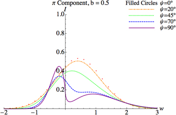
Figure 3. Same as in figure 2, but for b = 0.5.
Download figure:
Standard image High-resolution image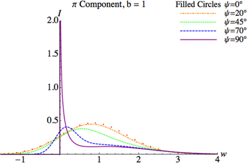
Figure 4. Same as in figure 2, but for b = 1.
Download figure:
Standard image High-resolution image
Figure 5. Same as in figure 2, but for b = 2.
Download figure:
Standard image High-resolution image
Figure 6. Same as in figure 2, but for b = 5.
Download figure:
Standard image High-resolution imageFigures 7–11 present the analogous set of Lorentz–Doppler profiles, but for σ-components of HHSL.

Figure 7. Lorentz–Doppler profiles of σ-components of highly-excited hydrogen/deuterium spectral lines calculated by equations (8) and (9), for the scaled magnetic field b = 0.2 (defined in equation (1)) at five different values of the angle of observation ψ with respect to the magnetic field.
Download figure:
Standard image High-resolution image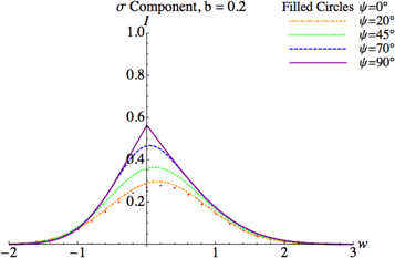
Figure 8. Same as in figure 7, but for b = 0.5.
Download figure:
Standard image High-resolution image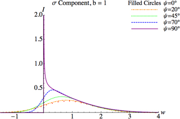
Figure 9. Same as in figure 7, but for b = 1.
Download figure:
Standard image High-resolution image
Figure 10. Same as in figure 7, but for b = 2.
Download figure:
Standard image High-resolution image
Figure 11. Same as in figure 7, but for b = 5.
Download figure:
Standard image High-resolution imageOne of the purposes of the present study was to see the evolution of the effect of the suppression of the π-components (compared to the σ-components) as the angle of the observation ψ decreases from 90°, i.e., as ψ decreases from the value, at which this effect was discovered in paper [1]. By comparing figures 7 and 11 (both of which correspond to b = 5, i.e., to the relatively strong magnetic field) we can deduce the following: as ψ decrease from 90° to 70°, the effect of suppression, while diminishing, is still present. However, already at ψ = 45°, the effect of the suppression is absent. Thus, we arrive to the conclusion that the suppression of the π-components (compared to the σ-components) occurs at the perpendicular or close to the perpendicular direction of observation (with respect to the magnetic field B), but rapidly disappears at lower values of the angle of the observation.
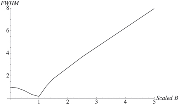
Another interesting result is in the following. The width of the Lorentz–Doppler profiles is a non-monotonic function of the scaled magnetic field b for observations perpendicular to B. As ∣b∣ increases from zero, the width first decreases, then reaches a minimum at ∣b∣ = 1 (i.e., when the shift in the Lorentz field is equal to the Doppler shift), and then increases—as presented in figure 12 using the Ly-beta line as an example. This is a counterintuitive result.
Figure 12. The Full Width at Half Maximum (FWHM) of the hydrogen/deuterium Ly-beta line observed perpendicular to the magnetic field B with a polarizer along B. The scaled magnetic field is the ratio of the Lorentz-field shift to the Doppler shift. The FWHM is in units of the Doppler half width at half maximum. The narrowing effect is the most pronounced when the Lorentz-field shift is equal to the Doppler shift.
Download figure:
Standard image High-resolution image
The decreasing part of the FWHM dependence on the magnetic field corresponds to relatively small magnetic fields: ∣b∣ < 1. In this range of ∣b∣, the line profile has the bell shape. In this range of ∣b∣, the complicated entanglement of the Doppler and Lorentz-filed mechanisms (that cannot be described as their convolution) causes the FWHM to decrease as ∣b∣ increases. This narrowing effect has a limited analogy with the well-known Dicke narrowing. Namely, in the Dicke case, the correlations between the Doppler mechanism and collisions cause the narrowing, while in our case the correlations (the complicated entanglement) between the Doppler mechanism and Lorentz-field mechanisms cause the narrowing. At relatively large magnetic fields, where ∣b∣ > 1, the line profile has the two-peak shape (one in the red part of the symmetric profile, another in the blue part of the symmetric profile). In this range of ∣b∣, the Lorentz-field mechanism dominates over the Doppler mechanism. Therefore, as ∣b∣ increases in this range, the two peaks of the profile move further apart and the FWHM increases.
3. Conclusions
We extended the analytical results for the Lorentz–Doppler profiles of HHSL for the arbitrary strength of the magnetic field B, obtained in paper [1] for observations parallel or perpendicular with respect to B, to arbitrary angles of the observation ψ. For this more complicated general case, we managed to reduce the analytical result to just a single integral.
We studied the evolution of the effect of the suppression of the π-components (compared to the σ-components) as the angle of the observation ψ decreases from 90°, i.e., as ψ decreases from the value, at which this effect was discovered in paper [1]. We found that the suppression of the π-components (compared to the σ-components) occurs at the perpendicular or close to the perpendicular direction of observation (with respect to the magnetic field B), but rapidly disappears at lower values of the angle of the observation.
We also found that the width of the Lorentz–Doppler profiles is a non-monotonic function of the magnetic field for observations perpendicular to B. This is a counterintuitive result.
The results of the present paper should be important, e.g., for spectroscopic diagnostics of edge plasmas of various magnetic fusion devices around the world—see, e.g., review [9] and references therein.
Footnotes
- 1
We note in passing that in paper [1] there were minor typographic errors in equations (31) and (32). In equation (31), the factor in front of the integral should be π−1∣2w∣−½. In equation (32), the factor in front of the last brackets should be [Γ(1/4)Γ(−1/4)]−1∣w∣−1/2.