


Abstract
Here, we analyze in natural time all earthquakes of magnitude (M) 3.5 or larger in Japan from 1 January 1984 until the occurrence of the super-giant M9 Tohoku earthquake on 11 March 2011. We find that two and a half months before this M9 earthquake a pronounced minimum of the entropy change of seismicity under time reversal is observed. Remarkably the exponent α resulting from the detrended fluctuation analysis of the earthquake magnitude time-series exhibits a simultaneous minimum with an unusual low value ( ) indicating an evident anticorrelated behavior. The validity of these findings is supported by the most studied non-conservative self-organized criticality model for earthquakes since it exhibts a non-zero change of the entropy upon time reversal, which reveals a breaking of the time symmetry, thus reflecting the predictability in this model.
Export citation and abstract BibTeX RIS
Introduction
The super-giant Tohoku earthquake (officially named Tohoku-chiho Taiheiyo-oki earthquake) of magnitude 9.0 that occurred in Japan on 11 March 2011 devastated the Pacific side of northern Honshu with a huge tsunami causing more than 20000 victims and serious damage of the Fukushima nuclear plant. This earthquake (EQ) was neither predicted for the short term nor the long term. Seismologists were shocked because it was not even considered possible that it might happen in the East Japan subduction zone. It is our main scope here to show that an important precursory change appeared almost two and a half months before this major EQ based on the main conclusion emerged in [1]. In particular, it has been shown [1] that upon analyzing the Olami-Feder-Christensen (OFC) model for EQs in a new time domain, termed natural time χ, a non-zero change  of the entropy in natural time upon time reversal is identified, which reveals a breaking of the time symmetry, thus reflecting the predictability in the OFC model. This model is probably [2] the most studied non-conservative, supposedly, self-organized criticality (SOC) model originated by a simplification of the Burridge-Knopoff (BK) spring-block model [3]. Ironically the SOC concept, originally introduced in ref. [4] using as an example the sandpile model (e.g., see also [5,6]) has been used as an argument that is not possible to predict the occurrence of large avalanches, e.g., see [2,7], based on the claim that avalanches seem to be uncorrelated in the original sandpile model. In other words, a belief was expressed that power-law distributed avalanches are inherently unpredictable, which came from the concept of SOC, but interpreted in the way that, at any moment, any small avalanche can eventually cascade to a large event. However, careful and detailed numerical studies [8,9] showed that particularly large events in a close to SOC system can be predicted on the basis of past observations. It is worthwhile to be noticed that the criticality of the OFC model has been debated (for example see [10,11]) and that the SOC behavior of the model is destroyed upon introducing some small changes in the rules of the model. For example introducing frozen noise in the local degree of dissipation [12] or in its threshold value [13], including lattice defects [14] —which should be distinguished from the intrinsic lattice defects in solids (e.g., see [15]). As for the EQ predictability [16] the OFC models appears to be closer to reality than others [17].
The present paper is structured as follows: In the next section, the background knowledge of natural time analysis is summarized along with the calculation of the entropy S in natural time together with the entropy  in natural time under time reversal. The Japanese seismicity data along with the details of the procedure followed in their analysis are described in the subsequent "Data and analyis" section and the results are presented in the fourth section. A brief discussion follows in the fifth section, while our main conclusions are summarized in the last section.
Natural time analysis and the change of the entropy under time reversal
For a time series comprising N events, we define an index for the occurrence of the k-th event by  , which we term natural time. In this analysis [18–22], we preserve the order of the events and their energy Qk because we consider that these two quantities are important for the evolution of the system. We, then, study the pairs
  , or the pairs
  , where
  is the normalized energy for the k-th event. Remarkably, natural time is currently considered as the basis for a new estimation of seismic risk by Turcotte and coworkers [23–26].
The entropy S in natural time is defined [19,27] as

where the bracket  denotes the average value of
  weighted by pk, i.e.,
  and
and  . It is dynamic entropy depending on the sequential order of events [28], thus changing upon the occurrence of each event. The entropy obtained by eq. (1) upon considering [29] the time-reversal
  , i.e.,
  , is labelled by
  , i.e.,

(see also [30,31]). The difference  will be hereafter labeled
  ; this may also have a subscript (
 ) meaning that the calculation is made (for each S and
  ) with a sliding window of length i (=number of successive events), i.e., at scale i (see also below). It has been shown [22] that
  , is probably a key measure which may identify when the system approaches the critical point (dynamic phase transition). For example,
  has been applied [32] for the identification of the impending sudden cardiac death risk (see also subsect. 9.4.1 of [22]) which is the major cause of death in industrialized countries [33–35]. Furthermore,
  was used as a useful tool [1] (see also subsect. 8.3.4 of [22]) to investigate the predictability of the OFC model. In particular, we found that the value of
  exhibits a clear minimum [22] (or maximum if we define as in [1]
  , instead of
  used here) before large avalanches in the OFC model. Thus, this minimum signals an impending large avalanche which corresponds to an impending large EQ.
As for the calculation of the time series of the entropy change under reversal, a window of length i (=number of successive events) was used, sliding each time by one event, through the whole time series. The entropies S and  , and therefrom their difference
  , were calculated each time. Thus, we form a new time series comprising successive
  values and search for their minimum which signals the occurrence of an impending phase change.
Data and analysis
The Japan Meteorological Agency (JMA) seismic catalogue was used (e.g., see [36,37]). We considered all EQs of magnitude  from 1984 until the Tohoku EQ occurrence on 11 March 2011 within the area 25°–46°N, 125°–146°E (yellow rectangle in fig. 1). The calculation was repeated also for a second larger area in order to avoid boundary effects and assure that the results do not depend on the selection of the area studied. Following [38] the eastern edge of the aforementioned area has been extended by 2° to the East, i.e., they also studied the area 25°–46°N, 125°–148°E shown by the black rectangle in fig. 1 for the following reason: The epicenter of a major EQ of magnitude 8.2 that occurred on 4 October 1994 lies inside the latter rectangle, but not in the former.

Fig. 1: (Color online) Map showing the two areas, larger 25°–46°N, 125°–148°E (black rectangle) and smaller 25°–46°N, 125°–146°E (yellow rectangle), in which the calculations of  values of seismicity during the period from 1 January 1984 until the M9 Tohoku EQ occurrence on 11 March 2011 were carried out. The star shows the epicenter of the M9 Tohoku EQ and the solid dot the one of the M7.8 EQ that occurred on 22 December 2010.
Download figure:
Standard imageThe energy of EQs was obtained from the JMA magnitude M after converting [39] to the moment magnitude Mw [40]. Setting a threshold  to assure data completeness, there exist 47204 EQs and 41277 EQs in the concerned period of about 326 months in the larger (black rectangle) and smaller (yellow rectangle) area, respectively. Thus, we have on the average
  and
and  EQs per month for the larger and smaller area, respectively.
The time evolution of  was studied for a number of scales i of the seismicity with
  occurring in both areas, larger and smaller, during the aforementioned almost 27 year period by selecting proper scales i as follows: We consider that recent investigations by means of natural time analysis showed that there exists the following interconnection between precursory low-frequency (
 ) electric signals, termed Seismic Electric Signals (SES), e.g., [41,42], and seismicity as follows [43]: The fluctuations β (e.g., see refs. [22,36]) of the order parameter
  of seismicity exhibit a minimum labeled
  when we observe the initiation of a series of consecutive SES termed SES activities [31,44,45] whose lead time ranges from a few weeks up to around
  months [22]. An SES activity, exhibiting critical behavior [18–20], is observed during a period in which long range correlations prevail between EQ magnitudes. On the other hand, before the initiation of the SES activity, and hence before
  , another stage appears in which the temporal correlations between EQ magnitudes exhibit an anticorrelated behavior [38] (as explained in more detail in our "Discussion" section below). Hence, there exists a significant change in the temporal correlations between EQ magnitudes when comparing the two stages that correspond to the periods before and just after the initiation of an SES activity. This change is likely to be captured by the time evolution of
  , thus we start our study of
  from the scale of
  events, which corresponds to the number of seismic events M ≥ 3.5 that occur during a period around the maximum lead time of SES activities.
Results
We start with the larger area 25°–46°N, 125°–148°E shown by the black rectangle in fig. 1 and we plot in fig. 2(a), (b), (c), (d), (e), (f) and (g), the  values vs. the conventional time for the scales
  ,
,  and
and  seismic events, respectively when analyzing all EQs with
  irrespective of their depth h during the period from 1 January 1984 until the occurrence of the M9 Tohoku EQ on 11 March 2011. In order to better visualize the change of the
  values when we approach the M9 Tohoku EQ occurrence, we also give in fig. 3(a), (b), (c), (d), (e), (f) and (g) an excerpt of fig. 2 but in expanded horizontal time scale during an almost
  month period from 1 October 2010 until the Tohoku EQ occurrence on 11 March 2011. We now turn to the smaller area 25°–46°N, 125°–146°E and plot in fig. 4(a), (b), (c), (d), (e), (f) and (g), in a similar fashion with fig. 2, the
  values vs. the conventional time for the same scales when analyzing the
  EQs irrespective of their depth during the period 1984–2011, while the corresponding
  month excerpt from 1 October 2010 until 11 March 2011 is given in fig. 5(a), (b), (c), (d), (e), (f) and (g).
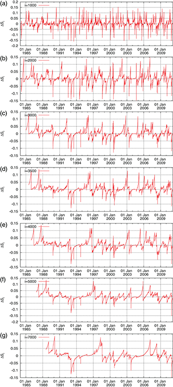
Fig. 2: (Color online) Plot of  values vs. the conventional time. Panels (a), (b), (c), (d), (e), (f) and (g) correspond to the scales
  ,
,  and
and  events, respectively, when analyzing all EQs with
  within the larger area 25°–46°N, 125°–148°E shown by the black rectangle in fig. 1 during the period from 1 January 1984 until the occurrence of the M9 Tohoku EQ on 11 March 2011.
Download figure:
Standard image
Fig. 3: (Color online) Excerpt of fig. 2 during the  month period from 1 October 2010 until the M9 Tohoku EQ occurrence on 11 March 2011. The higher two vertical lines ending at circles depict the magnitudes (
 ) read in the right scale that correspond to the M7.8 EQ on 22 December 2010 and the M9 Tohoku EQ on 11 March 2011.
Download figure:
Standard image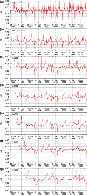
Fig. 4: (Color online) The same as fig. 2 but plotted for the smaller area 25°–46°N, 125°–146°E shown by the yellow rectangle in fig. 1.
Download figure:
Standard image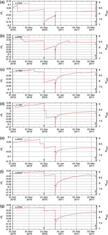
Fig. 5: (Color online) Excerpt of fig. 4 during the  month period from 1 October 2010 until the M9 Tohoku EQ occurrence on 11 March 2011. The higher two vertical lines ending at circles depict the magnitudes (
 ) read in the right scale that correspond to the M7.8 EQ on 22 December 2010 and the M9 Tohoku EQ on 11 March 2011.
Download figure:
Standard imageA careful inspection of figs. 2 and 4 for the larger and smaller area, respectively, reveals the following common feature: At shorter scales, i.e., from  to
to  events, a number of local minima appear, but leaving aside all these changes we find that at longer scales, i.e.,
  ,
,  and
and  events a pronounced minimum is observed on 22 December 2010. This date becomes more clear when focusing on fig. 3(a), (b), (c), (d), (e), (f), (g) and fig. 5(a), (b), (c), (d), (e), (f), (g) plotted in expanded time scale. We showed that the existence of this minimum is statistically significant, for example in the larger area, by the following procedure: We randomly shuffled the EQ magnitude time series and assigned each magnitude to an existing EQ occurrence time. We repeated the calculations 102 times and investigated the resulting
  time series of the longer scales, i.e.,
  ,
,  and
and  , for minima occurring on the same date and deeper than or equal to those depicted in fig. 2(e), (f), and (g), respectively. We found only 3 such cases out of the 102 studied. Hence, the probability to obtain minima comparable or deeper than those shown in fig. 2(e), (f), and (g) by chance is approximately 3% which shows that our result is statistically significant.
We now proceed to the investigation of the robustness of the appearance of this minimum on 22 December 2010 when changing the EQ depth, the magnitude threshold and the size of the area investigated. First, in order to investigate whether the EQ depth influences our result, we repeat the  values' calculations by considering only the shallow EQs, i.e., those with depth
  (in this case the number of EQs in the larger and smaller areas decrease from 47204 and 41277 EQs to 36834 and 31671 EQs, respectively). The corresponding results for the time evolution of
  values for the larger and smaller areas for shallow EQs are given in the Supplementary Material SupplementarymaterialPart1.pdf (SM1) in fig. S1(a), (b), (c), (d), (e), (f), (g) and fig. S2(a), (b), (c), (d), (e), (f), (g), respectively for the ∼27 year period 1984–2011 and their corresponding
  month period excerpts are depicted in fig. S1(h), (i), (j), (k), (l), (m), (n) and fig. S2(h), (i), (j), (k), (l), (m), (n), respectively. An inspection of these results reveals that the aforementioned common feature, i.e., the existence of a pronounced minimum on 22 December 2010, still pertains. Furthermore, this minimum remains on the same date if we repeat the calculation by also including intermediate EQs, 70–300 km deep, see figs. S3 and S4 (SM1) for the larger and smaller area, respectively. Second, concerning the magnitude threshold we find that the date of the minimum remains the same if we increase it from 3.5 used above to
  or
or  as can be seen in figs. S5 and S6, respectively, for the larger area and similarly in figs. S7 and S8 for the smaller area, see the SM1. Third, we show that the date of the minimum is not affected if we change the dimensions of the areas studied. In particular, beyond the two areas
  (larger, 25°–46°N, 125°–148°E) and
  (smaller, 25°–46°N, 125°–146°E) studied, we repeated the calculations for thirteen additional areas as follows: four areas with dimensions
  :
:  ,
,  ,
,  ,
,  , and nine areas with dimensions
  :
:  ,
,  ,
,  ,
,  ,
,  ,
,  ,
,  ,
,  ,
,  (see figs. S9, S10 in the SM1 and figs. S11–S21 in the Supplementary Material SupplementarymaterialPart2.pdf (SM2), respectively) and found the same date. The reason why the latter investigation was made for areas with dimensions around
  is shortly commented in the Discussion below.
Discussion
The following two comments are now in order as far as the date of the minimum of the  values identified on 22 December 2010 is concerned.
First, on this date the M7.8 Near Chichi-jima EQ occurred with an epicenter at 27.05°N 143.94°E [36,37].
Second, on the same date a significant change in the temporal correlations of the EQ magnitude time series in Japan has been observed: The magnitude time series before major EQs have been investigated in both areas (larger and smaller) shown in fig. 1 during the period 1984-2011 in ref. [38] by employing the Detrended Fluctuation Analysis (DFA) [46] which has been established as a standard method to investigate long range correlations in non-stationary time series in diverse fields (e.g., [46–57]). For each target EQ, the magnitudes of i = 300 consecutive events before the target have been analyzed [38] and a DFA exponent was therefrom deduced, hereafter labeled α, where  means random, α greater than 0.5 long range correlation, and α less than 0.5 anti-correlation. Focusing on the M9 Tohoku EQ under discussion, the calculations led to the following results [38]: the α values in both areas become markedly smaller than 0.5 after around 16 December 2010, including an evident minimum, i.e.,
  , on 22 December 2010. This was the lowest α value ever observed simultaneously in both areas during this ∼27 year period (cf. this anticorrelated behavior on 22 December 2010 is assured for all the aforementioned
  and
and  areas since we find α values lower than or equal to 0.37). From about 23 December 2010 until around 8 January 2011, the α values indicate the establishment of long range correlations since
  . In particular, during the last week of December 2010, the β values show that an evident decrease starts leading to a deep β minimum around 5 January 2011. This is the deepest
  observed [36] since the beginning of our investigation on 1 January 1984. Remarkably, the anomalous magnetic field variations [58], which accompany anomalous electric field variations, i.e., SES activities (see [59]), initiated almost on the same date, i.e., 4 January 2011, thus confirming the interconnection between SES and seismicity mentioned above in the "Data and analysis" section (since the SES activity started almost simultaneously with
  ).
).
We now shortly comment on the reason why our investigation on the area studied was made for areas with dimensions of around  . Tenenbaum et al. [60] proposed and developed a network approach to EQs. In this approach, a node represents a spatial location while a link between two nodes represents similar activity patterns in the two different locations. The strength of a link is proportional to the cross-correlation in the EQ activities of the two nodes joined by the link. They applied this network approach to the Japanese EQ activity during the period 1985–1998 by studying an area
  slightly exceeding the yellow area shown in fig. 1. Tenenbaum et al. [60] found strong links representing large correlations between patterns in locations separated by more than 1000 km (i.e., around 10° for mid-latitudes). Thus, in order to have such a situation through out a study area, it should have a "mean radius" of around 10° and hence dimensions around
  .
.
Main conclusions
Natural time analysis of seismicity in Japan during the almost 27 year period from 1 January 1984 until the occurrence of the M9 Tohoku super giant EQ on 11 March 2011 reveals that for longer scales, i.e., i > 3500 events, the minimum of  values is observed on 22 December 2010 simultaneously with the DFA exponent
  , which is the lowest exponent observed during the 27 year period of our study. This conforms to our earlier finding in [1] that before a large avalanche in the OFC model for EQs a minimum of the entropy change of seismicity under time reversal is observed.
Acknowledgments
The authors would like to express their gratitude to Professor Seiya Uyeda for repeated discussions on natural time analysis and Tohoku earthquake.