Abstract
Recent advances in three dimensional (3D) printing technology that allow multiple materials to be printed within each layer enable the creation of materials and components with precisely controlled heterogeneous microstructures. In addition, active materials, such as shape memory polymers, can be printed to create an active microstructure within a solid. These active materials can subsequently be activated in a controlled manner to change the shape or configuration of the solid in response to an environmental stimulus. This has been termed 4D printing, with the 4th dimension being the time-dependent shape change after the printing. In this paper, we advance the 4D printing concept to the design and fabrication of active origami, where a flat sheet automatically folds into a complicated 3D component. Here we print active composites with shape memory polymer fibers precisely printed in an elastomeric matrix and use them as intelligent active hinges to enable origami folding patterns. We develop a theoretical model to provide guidance in selecting design parameters such as fiber dimensions, hinge length, and programming strains and temperature. Using the model, we design and fabricate several active origami components that assemble from flat polymer sheets, including a box, a pyramid, and two origami airplanes. In addition, we directly print a 3D box with active composite hinges and program it to assume a temporary flat shape that subsequently recovers to the 3D box shape on demand.
Export citation and abstract BibTeX RIS
1. Introduction
Origami is a traditional art where a flat sheet of paper is folded into a complicated three dimensional (3D) shape. This art form emerged in the 1600s or earlier in countries such as Japan, China, Spain, Italy, and Germany, and has drawn significant interest in the art and mathematics communities since the 1940s and 1950s. Nowadays, origami is increasingly being explored to provide technological solutions to engineering problems of packing large objects into a small volume for storage or transport then deploying them for use, such as solar arrays in space structures or telescopes, airbags in automobiles, shopping bags and cartons (Dubey and Dai 2006, Merali 2011, Wu and You 2011), shape changing photovoltaic solar cells (Guo et al 2009, Myers et al 2010), and biomedical devices (Chalapat et al 2013, Gracias 2013, Hawkes et al 2010, Ionov 2011, Mahadevan and Rica 2005, Yang et al 2012). In these engineering applications, origami design can provide innovative solutions for ways to pack the material into its final form. But the packaging process itself is complex and presents automation challenges that may be unique to a specific packed configuration (Dubey and Dai 2006). These challenges increase the infrastructure cost, as a new automation infrastructure may be required if there are changes in the folding design. In addition, some folding patterns cannot be achieved by using regular folding processes. Active origami, where an object self-folds or self-unfolds, is therefore intriguing, as it can reduce the infrastructure investment for folding automations (Gracias 2013, Ionov 2011). Active materials, especially active polymers, are a natural choice for the design of active origami; e.g., origami using shape memory polymers (Liu et al 2012), light activated polymers (Ryu et al 2012), and shape memory alloys (Peraza-Hernandez et al 2013) were reported recently.
Recent developments in 3D printing enable the precise placement of multiple materials at micrometer resolution to create complex 3D configurations with no (or little) restrictions on the spatial arrangement of the materials. This unprecedented design freedom has motivated myriad studies and applications in science and engineering to create heterogeneous, designer materials with multiple functions. For example, Babaee used 3D printing to fabricate molds for casting spherical shells that are 3D metamaterials with negative Poisson's ratios due to local instabilities (Babaee et al 2013). The use of printed molds to cast spherical shells has also been employed to study buckling-induced encapsulation of structured elastic shells (Shim et al 2012) as well as the mechanics of nonspherical pressurized elastic shells (Lazarus et al 2012, Nasto et al 2013). Additionally, 3D printing has been used to directly fabricate heterogeneous materials. For example, Li et al (2013) fabricated soft multi-material polymer composites to investigate the mechanisms of the formation of wrinkled interfaces in soft multi-layered composites. Dimas et al (2013) printed fracture resistant composites that emulate biological composite topologies. In addition, 3D printing was used to create terahertz plasmonic waveguides (Pandey et al 2013), acoustic cloaks (Sanchis et al 2013), and medical devices (Khalyfa et al 2007, Lam et al 2002, Leukers et al 2005). Generally, 3D printing has been used as a fabrication technology to create 3D structures with complex details that cannot be created by other techniques (or are prohibitively expensive). Recently Tibbits introduced a new idea (Tibbits 2013), termed 4D printing, where a component is created by 3D printing but at a later time transforms into another shape or configuration. His materials and structures work by a hygroscopic effect, where the material swells in a temporally and spatially dependent manner when immersed in water. The different swelling ratios in regions made of different materials leads to deformation that conceptually can be designed to obtain a new configuration (Westbrook and Qi 2008). About the same time, Ge et al (2013) reported a paradigm of 4D printing to create printed active composites (PACs) by directly printing shape memory polymer fibers in an elastomeric matrix to enable programmable shape change of the composites. In the PAC system, the shape memory polymer (SMP) fibers, which are capable of fixing a temporary shape and recovering to their permanent shape in response to temperature change (Ge Luo et al 2012, Ge Yu et al 2012, Lendlein and Kelch 2002, 2005, Liu et al 2007, Mather et al 2009, Nguyen et al 2008, Qi et al 2008, Yu et al 2012), are critical to intelligentize the printed composite. The active composites are imbued with intelligence by thermomechanically programming a PAC lamina (printed fibers in a thin layer) or laminate (stacks of printed lamina) structure. After the thermomechanical programming (subjecting the material or structure to a prescribed thermal and mechanical loading profile), laminates designed and printed in a simple thin flat form assume complex 3D configurations including bent, coiled, and twisted strips; folded shapes; and complex contoured shapes with nonuniform, spatially-varying curvature. The resulting shape can be designed based on the theoretical understanding of the thermomechanical shape memory behavior of the composites and their constituents. The original flat form can be recovered by heating the material again. While the paper demonstrated the concept with simple printed flat laminate structures, more sophisticated shapes can be obtained by 4D printing, providing even more design freedom. For example, the two layer PACs can also serve as hinges connecting with rigid panels to create a self-folding/opening box. Potentially, the developed PAC hinges can play a striking role of making 3D self-assembly structures from a thin flat form.
In this paper, we advance the concept of self-assembling origami that works by printing flat polymer sheets connected by hinges consisting of PACs. When programmed with the appropriate thermomechanical protocol, the PAC hinges will fold the flat sheet into the desired final shape automatically, thus achieving active origami by 4D printing. Our approach is based on a rigorous understanding of the complex thermomechanics of the composite hinge structures and includes experiments to determine the folding angle of a hinge in terms of relevant microstructural parameters as well as a theory to describe the phenomena. With our theory, we can digitally design and manufacture components that can assemble themselves via active origami. In this paper, we first introduce the materials used to print PAC hinges then describe experiments to determine the hinge behavior as a function of the hinge PAC microstructural parameters and the thermomechanical loading parameters. In section 3, we develop a theoretical model to describe the bending angle of a PAC hinge as a function of the microstructure of the PAC composite and the thermomechanical constitutive behavior of the fibers and matrix. In our PACs, the matrix behaves as a simple elastomer, but the shape memory behavior of the PAC derives from that of the fibers, so we describe their behavior in the context of a thermomechanical constitutive model and characterize the relevant parameters. In section 4, we then use the understanding derived from our theory and experiments to design and manufacture by 4D printing a series of components that transform between two configurations: an as-printed initial configuration and an as-designed final configuration. These applications include a self-assembling box and pyramid that self-assemble from an initially flat shape, two origami airplanes that assemble into complex configurations from an initially flat shape, and a box that is printed in its 3D shape, deformed into a flattened temporary shape, and then re-assembled into its 3D box shape.
2. Printed active composite hinges—fabrication and characterization
2.1. Fabrication and materials
We fabricate PAC hinges by creating computer aided design (CAD) files that specify the complete 3D architecture of the fibers and matrix then printing them using a multi-material polymer 3D printer (Objet 260 Connex, Stratasys, Edina, MN, USA). The layer-by-layer printing process works by depositing droplets of polymer ink onto the building platform, wiping them into a smooth film, and ultraviolet (UV) photopolymerizing the film. Once a layer is created, the platform moves down, and the next layer is printed. Several inkjet heads with separate material sources exist in the printing block, so multiple materials can be printed in each layer. In our work, each layer generally contains materials that constitute part of the matrix and part of the fibers. In addition, a hydrophilic gel is printed and used as a sacrificial material for the fabrication of complex geometries (Stiltner et al 2011).
Our strategy to create PAC hinges consisting of composites with a matrix that is elastomeric over our desired operating temperature range of between room temperature and about 100 °C and fibers that exhibit the shape memory effect (SME) over this temperature range. Thus we design our PACs to have a matrix with a glass transition temperature  below 25 °C and fibers exhibiting SME in the range 25 °C–70 °C. To this end, we make use of the digital materials that are available with an Objet 3D printer. It provides two base materials: one is Tangoblack, a rubbery material at room temperature polymerized with a material ink containing urethane acrylate oligomer, Exo-1,7,7-trimethylbicyclo [2.2.1] hept-2-yl acrylate, methacrylate oligomer, polyurethane resin, and photo initiator; the other is Verowhite, a rigid plastic at room temperature polymerized with a material ink containing isobornyl acrylate, acrylic monomer, urethane acrylate, epoxy acrylate, acrylic monomer, acrylic oligomer, and photo initiator. The printer can also print digital materials that consist of varying compositions of these two materials that lead to different thermomechanical properties. In the current printing system, although users can tune thermomechanical properties of printed materials by choosing limited numbers of digital materials, we believe with the development of 3D printing technique, users will have more freedom of material choices. In this paper, we created PACs consisting of Tangoblack as the matrix (
 ∼ −5 °C) and a digital material (termed Gray 60) with
  ∼ 47 °C.
We created PAC hinges to characterize experimentally by directly printing two-layer PAC laminates that are connected to inactive (rigid) panels. These panels can be used as end tabs to apply mechanical loads (figure 1(a)). The PAC laminates consist of two layers: one layer of matrix-only material and one layer of a PAC lamina with a prescribed fiber size and spacing (figure 1(a)). The composite architecture is characterized by the lamina thicknesses and volume fraction (determined from the size and spacing).
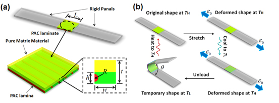
Figure 1. Schematics of a PAC hinge and the thermomechanical programming steps. (a) Geometrical and material properties of a PAC hinge. (b) Thermomechanical programming steps to train a self-folding/unfolding PAC hinge.
Download figure:
Standard image High-resolution imageOur hinges function via a mechanism of programmed strain mismatch (eigenstrain) between the two layers that leads to constant curvature bending over the hinge region, resulting in the plates on each side rotating an angle of  with respect to each other (figure 1(b)). The strain mismatch is created by: i) stretching the hinge at an elevated programming temperature (
 ,
,  >
>  ) to a prescribed strain (
 ), ii) cooling it to the usage temperature (
 ,
,  <
<  ) while maintaining the strain
  , and then iii) releasing the load. Upon releasing the mechanical constraint, the hinge bends to an angle
  due to the combined effect of the entropic elasticity of the pure matrix material lamina and the shape memory effect of the PAC lamina (Ge Qi et al 2013). The hinge returns to its original flat shape after heating back to
  .
.
2.2. PAC hinge behavior
We characterize the hinge performance by its bending angle  , which depends on the hinge materials (matrix and fiber thermomechanical constitutive behaviors), geometric parameters (hinge length L, and laminate/lamina configuration), and programming parameters (
 ,
,  , and
, and  ) (figure 1). In general our programming parameters are chosen so that rate effects do not play a role. In order to investigate the effects of these factors on hinge angle, we designed, fabricated, and carried out tests for a range of parameters including five different laminate/lamina configurations, three different programmed deformations (
 ∼ 10, 20, and 30%), and four different hinge lengths (
 = 2.5, 5.0, 7.5, and 10 mm). All of our tests were done with
  = 70 °C and
  = 25 °C. The laminate configuration is defined by the thickness of the hinge
  and the thickness of the PAC lamina
  . The PAC lamina is characterized by the fiber volume fraction
  , which we control by varying the fiber radius
  and the PAC lamina thickness
  , while keeping the fiber pitch fixed at
  = 1 mm. Table 1 shows the range of hinge parameters we used in our experiments. As described in section 3, we developed a theoretical model of the behavior of a PAC hinge, and this allows us to predict the result of hinge behavior beyond the range of parameters considered in our experiments.
Table 1. Geometrical parameters that describe PAC lamina and laminates.
| Case I | Case II | Case III | Case IV | Case V | |
|---|---|---|---|---|---|
| t (mm) | 0.6 | 0.6 | 0.6 | 0.5 | 0.5 |
| R (mm) | 0.125 | 0.1 | 0.1 | 0.1 | 0.08 |
| h (mm) | 0.3 | 0.3 | 0.2 | 0.2 | 0.2 |
 (%) (%) |
16 | 10 | 16 | 16 | 10 |
We carried out experiments to determine the behavior of the PAC hinges. Figure 2 shows hinge angles (measured at ∼1 min after unloading) as a function of the programming stretch and hinge length, respectively, for various laminate/lamina configurations. The results in figure 2(a) are for hinges with  = 5 mm and those in figure 2(b) for hinges with
  = 20%. Figure 2 demonstrates behaviors that are important to understand for the design of PAC hinges. For a fixed material and geometric configuration, the hinge angle decreases (the bending increases) with increasing programming stretch. This is simply because the mismatch strain between the layers increases with applied stretch, and this drives increased bending. Furthermore, as the length
  increases, the hinge angle decreases. This is also easy to understand, as the strain mismatch results in approximately constant curvature over the length of the hinge, and so geometry dictates a larger curvature (or smaller hinge angle
  ) as
) as  increases. More details regarding the behavior of the PAC hinges are presented in the following section in the context of a theoretical model we develop to describe the behavior.

Figure 2. The measured deformation of PAC hinges. (a) Hinge angle vs applied strain for 5 mm long hinges with five different cross-section profiles. (b) Hinge angle vs hinge length for hinges with five different cross-section profiles pre-stretched by 20%.
Download figure:
Standard image High-resolution image2.3. Thermomechanical testing
In order to obtain parameters used for the models developed in the next section, we also conducted a series of fundamental thermomechanical tests, including dynamic mechanical analysis (DMA) tests, uniaxial tensile tests, thermal strain tests, and stress relaxation tests.
We measured the storage modulus and tanδ vs temperature for the matrix and fiber materials (figure 3(a)) in uniaxial tensile tests performing on a DMA machine (TA Q800) (frequency = 0.1 Hz; cooling rate = 2 °C min−1; sample dimension 15 mm × 6 mm × 2 mm). In figure 3(a), within the temperature range from 100 °C − 50 °C, the storage modulus of the matrix soars from ∼0.7 MPa – ∼900 MPa, and that of the fiber soars from ∼6 MPa – ∼1.7 GPa. The peak of tanδ in the inset of figure 3(a) indicates the  of the matrix is ∼−5 °C, and the
  of the fiber is ∼47 °C.
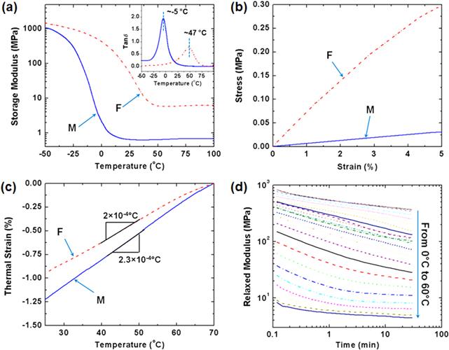
Figure 3. Thermomechanical tests for the matrix and fiber materials (M and F, respectively). (a) The results from DMA tests. (b) Uniaxial tensile tests at 70 °C. (c) Thermal strain tests. (d) Stress relaxation tests for the fiber material from 0 °C–60 °C with an interval of 2.5 °C.
Download figure:
Standard image High-resolution imageThe uniaxial tensile tests and thermal strain tests were also conducted on the DMA machine. The uniaxial tension tests were performed at 70 °C, where both the matrix and the fiber are at the rubbery state, and the samples with dimension 15 mm × 6 mm × 2 mm were stretched by 5% at a strain rate of 0.1%/s. In figure 3(b), the stress-strain behavior of the matrix and fibers shows a good linearity. Young's modulus of the fiber material is ∼6 MPa, while that of the matrix material is ∼0.7 MPa, which are consistent with those from the DMA tests. In the thermal strain tests, the termperature was descreased from 70 °C to 25 °C at a cooling rate of 2 °C min−1, under a constant tensile loading of 0.001 N to prevent samples from buckling. In figure 3(c), both the fiber material and the matrix material contract linearly with coefficient of thermal expansions (CTEs) 2 × 10⁻⁴ °C−1 and 2.3 × 10⁻⁴ °C−1, respectively. In figure 3(d), we also tested the stress relaxations for fibers at 25 different temperatures from 0 °C – 60 °C with an inteval of 2.5 °C, which are used to construct the stress relaxation master curve and fit parameters in the multi-branch model.
3. Theoretical estimates for PAC hinge behavior
Here we develop a simple but straightforward model to estimate the PAC hinge behavior; the model can then be used to guide the design of hinges. We first describe our modeling strategy to determine the curvature of the PAC hinge by combining a multilayer beam theory, homogenization, and the nonlinear time and temperature dependent constitutive behavior of the fibers and the matrix. We then introduce suitable constitutive behaviors for the fiber and matrix in the PAC. With parameters characterized from experiments, we use the developed model to estimate the hinge bending angle and compare the estimates with experimental results.
3.1. Hinge behavior—bending of a PAC bilayer laminate
For a material undergoing thermomechanical loading, the total deformation is due to both the thermal deformation (e.g., from thermal expansion/contraction, phase transformations, etc.) that if unconstrained does not give rise to stress and the mechanical deformation that gives rise to stress. The total deformation (or stretch, in the 1D case) of the material  (
( , where
  is the deformed length in the current state and
  is the original length in the reference state) can be decomposed into the mechanical deformation
  and the thermal deformation
  . That is,
  . For the sake of convenience, we use subscripts M and F to differentiate the deformations of the matrix or the fiber.
The bending of our hinges results from the mismatch strain between layers of the PAC laminate that arise from the shape fixing of the deformed shape memory fibers. As such, we model it as a two-layer laminate; one layer is simply an elastomer with properties of the matrix, and the other layer is a unidirectional fiber-reinforced lamina. To facilitate the analysis, we set Cartesian coordinates at the geometric center of the PAC laminate with the z-axis in the fiber direction, the y-axis downward, and the x-axis within the plane of the laminate (figure 4(a)). We consider the following thermomechanical loading steps: we uniaxially stretch the hinge at  , maintain the strain, cool it to
  , and then release the constraint.
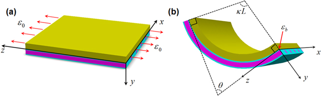
Figure 4. Schematics of achieving bending of a PAC hinges. (a) The flat PAC laminate is stretched by  at
at  and then cooled to
  while maintaining the strain
  . (b) After releasing the loading, the PAC laminate bends to a curvature
  (hinge angle
  ).
).
Download figure:
Standard image High-resolution imageDuring the first step, the sample is uniaxially stretched to 
 in a time period of
  at a constant stretch rate. Here, it is reasonable to assume that both the matrix and the fibers have the same strain, i.e.:
At  ,
,  . In the cooling step, let the cooling rate to be
  ; then the cooling time is
  . Both the matrix and fiber undergo thermal contraction, thus:

The formulations of the thermal deformations  will be introduced in equations (9) and (13), respectively.
Since the two ends of the hinge are fixed during the cooling, the total deformation (or stretch) does not change. This gives the mechanical deformations in the matrix and fibers as:

and the strains are
After releasing the constraint, the hinge bends with a curvature  . Due to bending, the midplane at
  undergoes a change in deformation (or stretch) by
  (figure 4(b)). Based on beam theory, other planes perpendicular to the y-axis deform by
  . Therefore, during bending, the total mechanical deformations (or stretches) in the matrix and fiber are:

Note that from the mechanics point of view, the hinge can be taken as a thin beam or plate. Therefore, although it can bend with a large rotation, the strain is usually small, and the Hencky strains are thus:
Since the bending occurs after releasing the external constraint, the total external force and total external moment applied to the hinge are zero (Dunn et al 2002, Ge Westbrook et al 2013, Westbrook Mather et al 2011):
In equation (6), the stresses on the matrix  and the fibers
  can be calculated through constitutive equations (8) and (10) introduced in the following subsections, by inputting the corresponding mechanical Hencky strains in equation (5). In equation (5), the variables
  ,
,  , and
, and  are measurable or calculable, but
  and
and  are two unknowns which can be calculated by solving equation (6).
Once the curvature  is calculated, the bending angle
  resulting from the geometrical relation (figure 4(b)) is:

In summary, to compute the curvature  and the bending angle
  , we first build up a set of two equations (equation (6)) to describe the total external force and total external moment. In the two equations, stresses on the fibers and matrix are calculated by their respective constitutive models, including measurable or calculable variables
  ,
,  ,
,  , and two unknowns
  and
and  . The two unknowns can be computed by solving the two equations in (6). Once the curvature
  is obtained, the bending angle
  can be calculated by equation (7). Using the developed model, we are able to describe the hinge bending angle as a function of the geometries, material constituents, and programming parameters.
Here, we note that the developed model is one dimensional, as it suffices to describe the operative deformation mode—bending of the hinges. The extension to 2D or 3D is important in general to extend the concepts here (tailored shape memory composite architectures in a laminated configuration) to more complex deformation modes, but it is not very important, in our opinion, to describe the deformation of the hinges in our work here. Indeed, we think this simplicity is somewhat elegant. The extension of the model to 2D or 3D is conceptually straightforward but practically challenging, as it will require nonlinear homogenization in 3D as well as characterization of the 3D constitutive behavior of the constituents. This would most likely be best done in a two-step approach (homogenization of the fibers and matrix within a layer followed by homogenization of the layers in the laminate) rather than in the combined manner we pursued here. As the goal of this model is to predict the macroscopic deformation of the laminate (curvature), we note a couple of treatments: (i) for simplicity we use a beam, rather than a plate, theory. We think this is warranted, given the simple deformation modes that our composite hinges exhibit; (ii) rather than homogenize each layer in the laminate (fibers and matrix) first and then proceed to model the laminate with its layers having effective homogenized properties, we homogenize within the layers (fibers and matrix) and throughout the laminate all in one step. This is tractable, given the 1D beam theory we adopt for simplicity, but in a full plate treatment it would probably be better to do each step separately. The end result is equivalent, though; (iii) in the homogenization of the fibers and matrix, we use a fairly sophisticated multi-branch constitutive model for the fibers that accounts for the nonlinear, time-dependent shape memory/fixing behavior as well as a simple hyperelastic model for the matrix. We realize that a more detailed model could be developed, at both the lamina level in terms of a fiber orientation distribution and inelastic behavior of the constituents (Dunn and Ledbetter 1997, Dunn et al 1996) and at the laminate level in terms of plate or even continuum behavior (Dunn et al 2002, Zhang and Dunn 2003, 2004), but we think the approach here is reasonable for understanding the basic behavior and designing components.
3.2. Thermomechanical constitutive behavior of the matrix
The matrix material shows entropic hyperelastic behavior over the operating temperature range of the hinge. Therefore, a simple hyperelastic model is adopted:

where  is the Hencky strain, which can be readily incorporated into the bending theory, and
  is the temperature dependent Young's modulus due to the entropic elasticity where
  is the cross-link density,
  is Boltzmann's constant, and
  is the absolute temperature. Based on our experimental observations (figure 3(c)), we describe the thermal deformation by a linear relation with the CTE of the matrix material
  :
:

3.3. Thermomechanical constitutive behavior of the fiber
The behavior of the fiber material over the temperature range is more complicated, as it exhibits the shape memory effect. To calculate the stress acting on the fiber material, we adopt a thermomechanical multi-branch model that decomposes the total deformation  into a mechanical deformation
  and a thermal deformation
  (Westbrook, Kao et al 2011, Yu et al 2014). For the mechanical elements in the model, an equilibrium branch associated with elastic response and several nonequilibrium branches associated with viscoelastic response are arranged in parallel. Each nonequilibrium branch is taken to be a Maxwell element, where an elastic spring and a dashpot are arranged in series. The total stress (Castro et al 2010, Ferry 1961) acting on the fiber material
  can be expressed as the sum of that in the equilibrium and nonequilibrium branches:
In equation (10), the first term is the stress from the equilibrium branch, where  is the temperature dependent Young's modulus and
  . The second term is the stress contribution from the nonequilibrium branches, where
  and
and  are the Young's modulus and the temperature dependent relaxation time for the mth branch.
  can be expressed in terms of
  and a temperature dependent shifting factor
  :
:

where  is the relaxation time for the mth branch at a reference temperature. Depending on whether the temperature is above, near, or below
  ,
,  is calculated by two different methods (O'Connell and McKenna 1999):
where  ,
,  , and
, and  are material constants,
  is the configuration energy,
  is Boltzmann's constant, and
  is the reference temperature.
Generally as a polymer goes through the glass transition from the equilibrium rubbery state to the nonequilibrium glassy state, the thermal deformation is a function of temperature as well as time. In addition, the dependence on time can become very weak (as the time constant for this dependence can be very long) as the time in the nonequilibrium state increases (Yu et al 2014). In the past, multiple theories (Kovacs et al 1979, Moynihan et al 1976, Robertson et al 1984) have been developed to represent the evolution of the nonequilibrium volume change. In this paper, we take a simple empirical approach based on our experimental observations. We represent the thermal deformation during the temperature change as:

where  is a linear thermal expansion coefficient of the fiber.
3.4. Parameter characterization
There are nine sets of parameters used in the thermomechanical constitutive models in total. They can be directly characterized by fitting the thermomechanical tests in section 2.
In the thermomechanical constitutive models for the matrix material, there are only two parameters, the crosslinking density  and CTE
  . By simply using equation (8),
  , to fit the uniaxial tensile test in figure 3(b) for the matrix material at 70 °C, one can readily have
  = 0.65 MPa and
  = 4.58 × 1025 m−3. Using equation (9),
  , to fit the thermal strain test in figure 3(c), we have
  = 2.3 × 10⁻⁴ °C−1.
Among the parameters in the multi-branch model in equation (10), the crosslinking density,  , can be readily identified by simply using
  to fit the stress-strain for the fiber material at 70 °C in figure 3(b), and
  = 4.23 × 1026 m−3. Stress relaxation tests in figure 3(d) were used to identify parameters in nonequilibrium branches. A stress relaxation master curve at 35 °C in figure 5(a) was constructed by shifting relaxation curves using shift factors
  at different temperatures (figure 5(d)). The master curve can be described by Maxwell elements in parallel, and the stress relaxation modulus is:
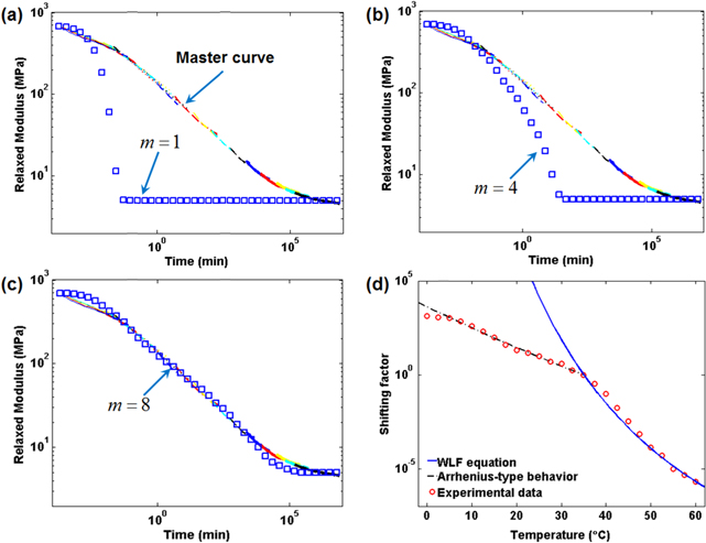
Figure 5. Model fitting for stress relaxation: (a)–(c) the stress relaxation master curve at 35 °C; (d) the shifting factors with temperature.
Download figure:
Standard image High-resolution imageIn equation (14),  is the relaxation modulus at time
  =
=  (
( ∼5 MPa in figure 5(a));
  is the relaxation time for the mth branch at the reference temperature (35 °C). We assume that the relaxation time of the mth branch is a decade longer than the (m-1)-th branch. At time
  = 0, the relaxation modulus is
  . Figures 6(a)–(c) present the model fitting for the stress relaxation. In figure 5(a), one nonequilibrium branch (
 = 1) was used to describe the stress relaxation modulus master curve. Based on equation (14),
  , one has
  (
( and
and  in figure 5(a). Through the observation of the stress relaxation master curve in figure 5(a), the obvious stress relaxation occurs at ∼0.006 min Here,
  was taken for the relaxation time of the first nonequilibrium branch. It is shown that an increasing number of nonequilibrium branches is required to precisely describe the stress relaxation modulus master curve. Figures 5(b) and (c) show the model fitting for the stress relaxation with
  = 4, 8 nonequilibrium branches, and the model fitting improves dramatically by introducing more nonequilibrium branches. Here, we take
  = 2 as an example to demonstrate the fitting procedure. In figure 5(a), at time
  , the discrepancy between the master curve and the model fitting is ∼250 MPa. This discrepancy can be corrected by introducing the second nonequilibrium branch with
  . Based on equation (14),
  , one has a new
  equal to 450 MPa. Assuming that the relaxation time of the second nonequilibrium branch is a decade longer than the first one, we have
  . Following the same fitting procedure, one has moduli for the all of the eight nonequilibrium branches (
 = 238 MPa,
  = 250 MPa,
  = 100 MPa,
  = 50 MPa,
  = 30 MPa,
  = 20 MPa,
  = 10 MPa, and
  = 2 MPa).
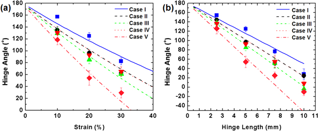
Figure 6. Model predictions of PAC hinge bending. (a) Hinge angle vs applied strain for 5 mm long hinges with five different cross-section profiles. (b) Hinge angle vs hinge length for hinges with five different cross-section profiles pre-stretched by 20%.
Download figure:
Standard image High-resolution imageThe parameters  ,
,  , and
, and  in equation (12) can be obtained by fitting the shift factor-temperature curve (figure 5(d)). Based on the experimental observation in figure 3(c), the CTE of the fiber material
  is 0.2 × 10⁻⁴ °C−1. All values of parameters in the constitutive models are listed in table 2.
Table 2. Lists of parameters for constitutive models.
| Parameter | Value | |
|---|---|---|
| Matrix material | ||
| Crosslinking Density |

|
4.58 × 1025 m−3 |
| CTE |

|
2.3 × 10⁻⁴ °C−1 |
| Fiber material | ||
| Crosslinking Density |

|
4.23 × 1026 m−3 |
| Elastic Moduli on Nonequilibrium Branches |
 , ,  , ,  , , 
 , ,  , ,  , , 
|
238, 250, 100, 50, 30, 20, 10, 2 MPa |
| Relaxation Time of the 1st Branch |

|
0.36 s |
| WLF constant |

|
17.66 |
| WLF constant |

|
51.6 °C |
| Pre-exponential parameter |

|
−20000 K |
| CTE |

|
0.2 × 10⁻⁴ °C−1 |
3.5. Theoretical estimates and discussions
As introduced in 3.1, the curvature  and the midplane strain
  can be solved by incorporating the constitutive equations for the matrix and fibers from equations (8)–(13) with the corresponding mechanical Hencky strains in equation (5) into equation (6) (Details are straightforward, although tedious, and are shown in the appendix):

In composite laminate mechanics,  ,
,  , and
, and  are termed the extensional stiffness, coupling stiffness, and bending stiffness, respectively. If the laminate is symmetric with respect to the geometric midplane, then
  = 0 (in our case it is not by design).
  and
and  are called the thermal force and moment, respectively. Here they arise from the mismatch strain between layers in the laminate due to the shape fixing of the shape memory fibrous lamina; they are the driving force for the bending of the hinge. Equation (15) yields the curvature of the laminate:

Once the curvature  is calculated, the bending angle
  can be directly obtained by equation (7).
With the characterized parameters listed in table 2, we use our model to plot the predicted hinge angle vs applied strain at  (figure 6(a)), and the hinge angle vs the hinge length (figure 6(b)) for the five different cross section profile cases of table 1. Table 3 shows the predicted laminate parameters (A, B, D,
  , and
, and  ) for the laminate, with
  and
and  computed for an applied strain of 30%. It is noted that as
  and the curvature
  are time dependent; all laminate parameters are computed at 1 min after unloading.
Table 3.
Laminate thermomechanical parameters that determine the hinge angle of a PAC laminate. (All parameters are computed at 1 min after unloading.  and
and  are computed at an applied strain of 30%).
| Case I | Case II | Case III | Case IV | Case V | |
|---|---|---|---|---|---|
 
|
4.63 | 3.02 | 3.02 | 2.99 | 1.97 |
 
|
0.67 | 0.43 | 0.57 | 0.43 | 0.27 |
 
|
0.12 | 0.076 | 0.13 | 0.074 | 0.047 |
 
|
−0.078 | −0.066 | −0.066 | −0.059 | −0.051 |
 
|
−0.0048 | −0.0031 | −0.0059 | −0.0031 | −0.002 |
The hinge behavior as a function of applied strain and hinge length is easy to understand, but its behavior in terms of other microstructural parameters, e.g., cases I-V, is less straightforward to understand. Composite laminate mechanics provide a convenient way to understand the behavior of the PACs in terms of the microstructural parameters, specifically as it is expressed through the variation of A, B, D,  , and
, and  . These are a function of the applied strain but reported for
  = 30% in table 3. In essence, the five cases in table 3 systematically vary the volume fraction of the SMP fibers in the PAC lamina and the thicknesses of the two lamina that make up the laminate. Here we make a few observations important for the design of PAC hinges, based on our experiments and theory:
- Compared to Case I, the Case II hinge bends more because of the lower fiber volume fraction, with the lamina thicknesses equal.
- In Case III, the hinge bends more than that in Case II as the thickness of the lamina with the SMP fibers decreases, even though the volume fraction increases.
- The behavior of Case IV is comparable to that of Case II, and this arises because of the combination of the higher volume fraction for Case IV and the smaller thickness of lamina, and thus laminate.
- Case V, with the lowest fiber volume fraction and the thinnest lamina (and most compliant laminate) bends the most.
The hinge bending results from the interplay among the laminate parameters A, B, D,  , and
, and  , which represent the effects of the microstructural parameters on the collective behavior of the shape memory fibers and the elastomeric matrix that contribute to produce the applied loading and laminate stiffness. Table 3 shows that the coupling between extension and bending (represented by the stiffness B and its role in equation (16)) significantly influences the bending of the laminate and the resulting hinge angle. Indeed it is through this coupling that our hinges operate as we apply a tensile strain. Via the internal workings of the lamina and laminate architecture, the laminate bends. Our results demonstrate that PAC laminate hinges can be designed to exhibit a controlled hinge angle, but because of the numerous design variables and their interacting influence, their design benefits greatly from a theory that can describe the observed behavior.
4. Creating printed origami
We created a number of examples that demonstrate how we can print flat-plate structures consisting of PAC hinges directly connected to rigid plastic components of arbitrary shape then program the hinges to assemble the as-printed structure into a desired 3D configuration. As we showed, composite hinges can be programmed to assume prescribed folding angles, and these depend on a set of material, geometrical, and programming parameters. As such, here we use our experimentally validated model to design the hinge parameters for a range of applications.
First we designed a box consisting of six sides connected by PAC hinges that is printed in a flat (unfolded) form as shown in figure 7(a). The hinges were designed by choosing parameters from figure 6(a) that result in a hinge angle of 90°. Specifically, we created hinges from PACs with parameters from Case III of table 1 and stretched the box biaxially by 20%. Figure 7(a) shows the as-printed box (the flat plate), where the rigid sides are white and the hinges are black. The assembled box was created after biaxially stretching the as-printed structure by 20% at  , cooling to
  , and releasing the load. It clearly assembles into the desired box shape (figure 7(b)), with only small deviations from the desired 90° angles, and these are likely due to inaccuracies in the straining process.
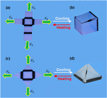
Figure 7. Active origami box and pyramid. The printed flat cross shape in (a) assembles itself into a desired box shape in (b) after the programming steps. The printed flat Ninja star shape plate in (c) assembles itself into a desired pyramid shape in (d) after the programming steps.
Download figure:
Standard image High-resolution imageFigure 7(c) and d show a similar structure, a five-sided 3D pyramid. Here the printed flat Ninja star shape plate consists of a square base with four triangular sides (figure 7(c)) that are folded to 3D pyramids with 60° angles (figure 7(d)). We create the printed Ninja star shape using hinges from Case V of figure 6(c) with a programming stretch of 20%. Again, the desired 3D shape is in good agreement with the intended shape.
We can also create complex 3D shapes with different hinge angles by printing hinges with different geometries. Figure 8(a) shows a flat triangle sheet that folds itself into an origami airplane with a 0° angle in the middle hinge that bends upward and 90° angles in the two side hinges that bend downward. To realize such an assembled configuration, we printed a 7.5 mm hinge (Case V in figure 6(b)) in the middle and two 4 mm hinges (Case V in figure 6(b)) on the two sides and stretched the flat triangle sheet by 20%. The hinges are created by printing the bilayer composites with the fibers on the top layer for the 0° hinges and on the bottom for the 90° hinges. To simplify the loading process (allowing simply a 20% stretch), we print the 90° hinges in figure 8(a) at an inclined angle relative to the base of the plane, but we maintain the fiber orientations parallel to the base (and the applied stretch, figure 8(a) inset). We create an even more sophisticated origami airplane by printing not only hinges with different lengths but also ones with different cross-section profiles (figure 8(b)). Here the origami airplane has two winglets created by printed hinges designed to bend 120° upwards (4 mm long Case IV hinges in figure 6(b)).
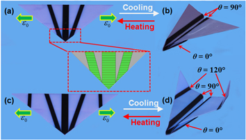
Figure 8. Active origami airplanes. A flat triangle sheet with three hinges in (a) assembles itself into an origami airplane with a 0° angle in the middle hinge that bends upward and 90° angles in the two side hinges that bend downward in (b). A flat triangle sheet with five hinges in (c) assembles itself into an origami airplane with two winglets in (d).
Download figure:
Standard image High-resolution imageThe relationships among the hinge parameters (hinge angle, stretching strain, hinge length) for the five cross-section profile cases provide valuable information to design a desired hinge angle with a combination of stretching strain, hinge length, and one of the cross-section profile cases. Of course, the options for the cross-section profile are not limited to the five cases presented in this paper. Depending on the application, a strategy might involve using a few parameters to define the cross-section profile then adjusting the applied stretch and hinge length to achieve a desired hinge angle. In fact, the advantage of PACs is that the choice of the combination of these parameters to obtain a particular hinge angle can be large, thus allowing considerable design flexibility. Of course, the most powerful is the ability to use our model to design the hinge parameters, including the temperature range, with minimal experiments.
The use 3D printing of active materials to create components that controllably change their shape over time is not limited to the use of PAC hinges. In fact, we can directly print 3D devices by strategically placing shape memory polymers at pivotal locations or throughout an entire structure. We can then program a temporary shape of arbitrary form that can be achieved by applying a prescribed mechanical loading at  followed by releasing the constraints at
  . The components can then be returned to their complex original 3D shapes after heating back to
  . Figure 9 shows such an example. We directly printed a 3D box with a pattern of SUTD-CU logos on the five panels. In figure 9(a), the complete 3D box is printed with a three-layer laminate consisting of a Verowhite middle layer embedded in a Tangoblack matrix. The box is then deformed to a flat form (figure 9(b)) by applying mechanical loads at
  , and cooled to
  where the constraints were removed, leaving it in a flat form. Upon heating back to
  , the structure retakes the original 3D box shape (figure 9(a)).
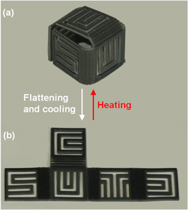
Figure 9. A directly printed origami SUTD-CU box. An as-printed 3D SUTD-CU box in (a) was deformed into a flat form at  in (b). After heating back to
  , the structure recovers the 3D box shape.
Download figure:
Standard image High-resolution imageCompared to the means of printing flat components with PAC hinges and then assembling them into 3D components, directly printing 3D components with SMPs allows the creation of complex 3D configurations that are potentially more precisely controlled, as they are printed directly in their permanent shapes. However, the direct printing requires longer manufacturing times and uses more material than printing flat components and assembling them. For example, the fabrication time depends on the thickness dimension of the printed object, since it is created in a layer-by-layer process. With the Objet printer used in this work, a 1 mm thick structure takes roughly 10 mins to complete. Creating a 20 mm × 20 mm × 20 mm box requires only about 10 mins to print the ∼1 mm thick flat sheet with PAC hinges that can then be assembled as in figure 8(a), but it takes about three hours to print the 3D box directly (e.g., figure 9). Furthermore, to support the upper part of the 3D box, a large amount of sacrificial material is used. The process to remove the sacrificial material can also take several hours, depending on the complexity of the structure.
5. Conclusions
In this paper, we furthered the 4D printing concept to enable active origami as a means of creating 3D components. In our approach, we printed 2D flat sheets with hinges created by composites with polymer fibers. These fibers exhibit the shape memory effect over a desired operating temperature range in an elastomeric matrix. By a suitable thermomechanical programming process, we actuated the hinges, making them fold to a prescribed angle and, as a result, folding the 2D sheet into a 3D structure. The folding of the printed composite hinges depends on the material properties of the polymers (including the shape memory behavior of the fibers), the lamina and laminate architecture, and the thermomechanical loading profile. We developed a theoretical model to describe the behavior of the printed active composite hinges and used it to design several active origami structures, including a self-assembling box and pyramid and two origami airplanes. While our design parameters here were limited to composite hinges placed at locations where we desired folding, a more flexible approach based on topology optimization with active materials could be used in more general situations (Howard et al 2009, Pajot et al 2006). Finally, we also demonstrated the direct printing of a complex 3D structure that can then be programmed to assume a simpler temporary shape (a flat sheet in our case) and then recover its original 3D shape.
Acknowledgement
We gratefully acknowledge the support of an AFOSR grant (FA9550-13-1-0088; Dr B.-L. 'Les' Lee, Program Manager). HJQ acknowledge the support of the NSF award (CMMI-1334637 and EFRI- 1240374). MLD acknowledges support from the MOE of Singapore and the SUTD-MIT International Design Centre.
Appendix A.: Solution for the PAC bilayer laminate bending
Equations (8) and (10) in section 3 expressed the stresses on matrix and fibers in any plane perpendicular to the y-axis, including two unknowns  and
and  . Here, we first convert them from the calculus form to summation form:
Here,  is the mechanical Hencky strain at time
  before unloading and
  . During unloading at time
  , the planes perpendicular to the y-axis away from the origin with
  deforms by
  .
.
In order to reduce the difficulty in solving equation (6), the mathematical treatments were made to separate  and
and  from other terms in equation (A1). For the stress on the matrix, we simply separate the parts before unloading (at
  ) and during unloading (at
  ):
):
where  is the stress before unloading and denoted as
  for brevity.
  is the stress during unloading, and
  is denoted as
  . For the stress on fibers, to separate
  and
and  from other amounts, we have:
where  is the stress on the equilibrium branch before unloading (at
  ), and
 ![$\sigma _{m}^{k}=E_{non}^{m}\mathop \sum \nolimits_{i=1}^{k} \left[ \Delta e_{F}^{i}\mathop \sum \nolimits_{j=i}^{k} {\rm exp} \left( -\frac{\Delta {{t}_{j}}}{\tau _{m}^{j}} \right) \right]$](https://content.cld.iop.org/journals/0964-1726/23/9/094007/revision1/sms495700ieqn233.gif) is the stress on the mth nonequilibrium branch before unloading (at
is the stress on the mth nonequilibrium branch before unloading (at  ). The detailed derivation for equation (A2b) is listed in appendix B.
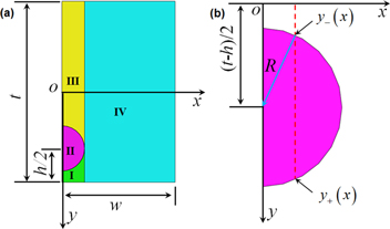
As the laminate consists of different materials within different geometries, we divide the cross-section into four sub-regions (figure 10(a)): I. the part right beneath the fiber consists of the matrix material (the green part in figure 10(a)). II. The semi-circular fiber (the purple part in figure 10(a)). III. The part right above the fiber consists of the matrix material (the yellow part in figure 10(a)). IV. The remaining part consists of the matrix material (the blue part in figure 10(a)). The upper and lower y coordinates on the semi-circular fiber are (figure 10(b)):

Figure 10. Schematics of the cross-section of a PAC laminate. (a) The cross-section is divided into four sub-regions. (b) The semi-circular fiber is broken into  segments.
Download figure:
Standard image High-resolution image
We calculate the forces in the sub-regions I–IV ( ,
, ,
, , and
, and  ) by using the stress forms in equations (A2a) and (A2b):
As in equation (6) the total external force is zero  . We have:

where  and
and  and
and  .
.
Also, we calculate the moments in the sub-regions I–IV ( ,
, ,
, , and
, and  ) by using the stress forms in equations (A2a) and (A2b):
As in equation (6) the total external force is zero  . We have:

where  and
and  .
.
The midplane strain  and the curvature
  can be solved by using equations (A4b) and (A4d):

Appendix B.: Detailed derivation for equation (A2b)
At time  , when it is cooled to
  , but the strain constraint is still on, we have the stress on the fibers in the summation form:
where  is the stress on the equilibrium branch and
  is the nonequilibrium stress on the mth branch.
At time  , a strain
  is released. Similar to equation (A6), we have the stress on the fibers:
Through equation (A7a), we can separate  and
and  from
from  :
: