
Abstract
Low-stabilization scenarios consistent with the 2 °C target project large-scale deployment of purpose-grown lignocellulosic biomass. In case a GHG price regime integrates emissions from energy conversion and from land-use/land-use change, the strong demand for bioenergy and the pricing of terrestrial emissions are likely to coincide. We explore the global potential of purpose-grown lignocellulosic biomass and ask the question how the supply prices of biomass depend on prices for greenhouse gas (GHG) emissions from the land-use sector. Using the spatially explicit global land-use optimization model MAgPIE, we construct bioenergy supply curves for ten world regions and a global aggregate in two scenarios, with and without a GHG tax. We find that the implementation of GHG taxes is crucial for the slope of the supply function and the GHG emissions from the land-use sector. Global supply prices start at $5 GJ−1 and increase almost linearly, doubling at 150 EJ (in 2055 and 2095). The GHG tax increases bioenergy prices by $5 GJ−1 in 2055 and by $10 GJ−1 in 2095, since it effectively stops deforestation and thus excludes large amounts of high-productivity land. Prices additionally increase due to costs for N2O emissions from fertilizer use. The GHG tax decreases global land-use change emissions by one-third. However, the carbon emissions due to bioenergy production increase by more than 50% from conversion of land that is not under emission control. Average yields required to produce 240 EJ in 2095 are roughly 600 GJ ha−1 yr−1 with and without tax.
Export citation and abstract BibTeX RIS

Content from this work may be used under the terms of the Creative Commons Attribution 3.0 licence. Any further distribution of this work must maintain attribution to the author(s) and the title of the work, journal citation and DOI.
1. Introduction
Energy from biomass as a substitute for fossil energy is not only supposed to improve energy security. Several studies investigating the transition of the energy system under climate change stabilization targets consider bioenergy a large-scale and cost-effective mitigation option (Riahi et al 2007, Calvin et al 2009, Luckow et al 2010, Van Vuuren et al 2010a, Rose et al 2013). In particular, bioenergy with CCS (BECCS) may significantly reduce stabilization costs, since its negative emissions compensate emissions from other sources and across time (Van Vuuren et al, 2010b, 2013, Kriegler et al 2013, Azar et al 2010, 2013, Klein et al 2013). The amount of realizable negative emission directly depends on the amount of biomass available. Thus, the biomass potential and its cost become crucial factors that affect overall mitigation costs (Rose et al 2013, Klein et al 2013). While the scientific consensus on the importance of bioenergy for climate change mitigation is strong (Rose et al 2013), high uncertainties remain regarding the biomass potential, resulting in wide ranges of estimates (28–655 EJ yr−1, see also section 2). This is mainly due to uncertainties about future developments of agricultural yields1 , demand for food and feed, and availability of land and water for agricultural production. In particular, there are only a few global studies attributing costs or prices to the estimated bioenergy potential (see also section 2). The purpose of this study is to provide supply price curves for lignocellulosic biomass that can serve as a basis for the economic assessment of bioenergy in climate change mitigation scenarios.
Low-stabilization scenarios consistent with the 2 °C target project large-scale deployment of biomass necessitating dedicated production of modern lignocellulosic biomass at levels that exceed the potential of residues and first-generation biofuels (Popp et al 2013). Therefore, this study focuses on purpose-grown lignocellulosic and herbaceous biomass. A major concern about the sustainability of large-scale bioenergy production is its potential to induce deforestation. First, deforestation causes carbon emissions and counteracts the objective of emission mitigation if no effective forest protection regime is in place (Wise et al 2009, Popp et al 2011a, 2012, Calvin et al 2013). Second, deforestation entails substantial biodiversity loss, as forests are the most biologically diverse terrestrial ecosystems (Turner 1996, Hassan et al 2005). Both adverse effects could be considerably mitigated if GHG emissions from the land-use sector (including non-CO2 emissions such as N2O from fertilizer use) were equally priced with energy emissions. In the case of a GHG price regime comprising energy and land-use/land-use change emissions, the strong demand for bioenergy and pricing of terrestrial emissions are likely to coincide, and the GHG pricing is likely to affect the availability and productivity of land for bioenergy, and thus bioenergy prices for a given level of demand. However, to our knowledge the available literature on bioenergy potentials does not consider GHG pricing in the land-use sector (Hoogwijk 2004, Hoogwijk et al 2005, 2009, Smeets et al 2007, Erb et al 2009, Van Vuuren et al 2009, Dornburg et al 2010, Haberl et al 2010, Beringer et al 2011a). Therefore, this study investigates the impact of GHG prices on the potential and the supply prices of bioenergy.
Furthermore, these studies assume bioenergy production only on land not required for food production, and they assume yield improvements to be independent of bioenergy demand. However, these assumptions may not hold if the demand for bioenergy strongly increases, as projected by low-stabilization scenarios. In contrast, the approach applied for this study incorporates land competition between bioenergy and other crops. Moreover, it allows derivation of yield improvement rates required to satisfy given levels of bioenergy and food demand, since technological development is endogenous in this approach. Using the land-use optimization model MAgPIE (Model of Agricultural Production and its Impacts on the Environment) (Lotze-Campen et al 2008, Popp et al 2010), we construct bioenergy supply curves for ten world regions by measuring the bioenergy price response to different scenarios of bioenergy demand and GHG prices. The model endogenously treats the trade-off between land expansion (causing costs for land conversion and for resulting carbon emissions) and intensification (requiring investments for research and development) by minimizing the total agricultural production costs. GHG emissions from the land-use system are priced, and resulting costs for emissions accruing from bioenergy production are reflected in bioenergy prices.
The purpose of this study is to quantitatively assess the global economic potential of lignocellulosic purpose-grown biomass under different climate policy proposals. It presents bioenergy supply price curves on a regional level. Two key questions are addressed: what is the global potential of purpose-grown second-generation biomass and how are potential and corresponding supply prices dependent on GHG taxes?
2. Present bioenergy potential studies
It is important to note that this study focuses on second-generation biomass. The literature about first-generation biomass is larger, but not a concern here. Several studies have investigated the global potential of second-generation purpose-grown bioenergy under different constraints. There are mainly two types of global bioenergy potential study so far. The first group identifies the potential of bioenergy by defining the area of land available for bioenergy production and by making assumptions about the productivity of this land (Hoogwijk et al 2005, Smeets et al 2007, Erb et al 2009, 2012, Van Vuuren et al 2009, Dornburg et al 2010, Haberl et al 2010, 2013, Smith et al 2012, Beringer et al 2011a). These studies assume some kind of food-first policy, as they exclude land that is needed for food and feed production and allow bioenergy production only on land that is not used for food production or might in future become available due to intensification or decreasing demand for agricultural commodities. The development of technological change is included in these studies by exogenous assumptions on food and feed crop yield growth that largely determine the land available for bioenergy production. Other important factors are food demand, trade, and livestock production. Some studies consider additional sustainability constraints by excluding land for forest and nature conservation or due to water scarcity or degradation (Van Vuuren et al 2009, Beringer et al 2011a). Based on these studies, the estimates of the purpose-grown biomass potential for 2050 range from 28–265 EJ yr−1 at the lower end to 128–655 EJ yr−1 at the upper end2 .
The wide range can be explained by different assumptions on food demand, availability of land, and development of yields, which are identified by these studies as the main determinants of the bioenergy potential. Low estimates are mainly driven by assuming high population growth (resulting in high food demand) and excluding water scarce areas and nature conservation areas, resulting in low availability of land for bioenergy production. Projected future yields are another crucial (yet highly uncertain) parameter determining the bioenergy potential. Haberl et al 2010 report a wide range of 7–60 GJ ha−1 yr−1 used in the literature. The estimates at the upper end of bioenergy potentials are mainly based on high-yield growth rates for food and bioenergy crops over the next decades that are at present level or higher (Hoogwijk et al 2005, Van Vuuren et al 2009, Smeets et al 2007, Dornburg et al 2010).
These studies use simulation models to project the future development of the land-use system and feature different levels of spatial explicit biophysical conditions. The projections applying average yields over large areas considered suitable for bioenergy production tend to project high bioenergy potentials, 120–660 EJ yr−1 (Hoogwijk et al 2005, Van Vuuren et al 2009, Smeets et al 2007, Dornburg et al 2010), while process-based studies that aim to include spatially explicit data on local biophysical conditions estimate lower ranges, 37–141 EJ yr−1 (Beringer et al 2011b, Erb et al 2009, 2012). Another approach derives the actual net primary productivity (NPP) from satellite data and argues that the NPP poses an upper bound to bioenergy production. The estimates reported by these studies (excluding residues) are 121 (Smith et al 2012) and 190 (Haberl et al 2013).
However, to be able to assess the economic potential and hence the competitiveness of bioenergy in the energy system, one needs information about the supply costs of biomass. Therefore the second group of studies additionally assigns costs for bioenergy production to the different types of land cell and constructs supply cost curves by sorting the cells by their biomass production costs. Only a few studies provide information about the production costs, particularly concerning second-generation bioenergy on a global scale (Hoogwijk 2004, Hoogwijk et al 2009, Van Vuuren et al 2009). Hoogwijk (2009) introduces costs for land, capital, and labor to the technical potential identified in Hoogwijk (2005) and finds that 130–270 EJ yr−1 in 2050 may be produced at costs below $2.2 GJ−1 and 180–440 EJ yr−1 below $4.5 GJ−1 3 . The underlying scenarios assume significant land productivity improvements and cost reductions due to learning and capital–labor substitution. Using a similar approach (but assuming less available land due to a lower accessibility factor), Van Vuuren et al (2009) excludes further areas from biomass production due to biodiversity conservation, water scarcity, and land degradation. This reduces the global biomass potential in 2050 from 150 EJ yr−1 without these land constraints to 65 EJ yr−1. Following the same cost approach as Hoogwijk (2005), Van Vuuren et al (2009) finds that in 2050 about 50 EJ could be produced at costs below $2.2 GJ−1 and 125 EJ below $4.8 GJ−1. Realizing the full potential of 150 EJ by taking biomass from degraded land into account would cost up to $8 GJ−1. Both studies allow bioenergy production on abandoned and rest land only and consider only woody bioenergy crops.
3. Methods
3.1. The land-use model MAgPIE
MAgPIE is a spatially explicit, global land-use optimization model (Lotze-Campen et al 2008, Popp et al 2010). The objective function of MAgPIE is the fulfillment of food, livestock, material, and bioenergy demand at least costs under socio-economic, political, and biophysical constraints. Demand is income elastic, but price-induced changes in demand are not reflected. Major cost types in MAgPIE are factor requirement costs (capital, labor, and fertilizer), land conversion costs, transportation costs to the closest market, investment cost for technological change (TC), and costs for GHG emission rights. The cost minimization problem is solved in 10-year time steps until 2095 in recursive dynamic mode by varying the spatial production patterns, by expanding crop land, and by investing in yield-increasing TC (Lotze-Campen et al 2010, Dietrich et al 2012). TC increases the potential yields of all crops within a region by the same factor. The costs for enhancing the yields in a specific region increase with the level of agricultural development of the particular region; i.e., the higher the actual yields in a region the higher the costs for one additional unit of yield increase (Dietrich et al 2014). The model distinguishes ten economic world regions with global coverage (cf supplementary material section S1.2): Sub-Saharan Africa (AFR), Centrally Planned Asia including China (CPA), Europe including Turkey (EUR), states of the former Soviet Union (FSU), Latin America (LAM), Middle East/North Africa (MEA), North America (NAM), Pacific OECD including Japan, Australia, New Zealand (PAO), Pacific (or Southeast) Asia (PAS), and South Asia including India (SAS). MAgPIE considers spatially explicit biophysical constraints such as crop yields and availability of water (Bondeau et al 2007, Müller and Robertson 2013) and land (Krause et al 2013) as well as socio-economic constraints such as trade liberalization, forest protection, and GHG prices.
MAgPIE differentiates between the land types cropland, pasture, forest, and other land (e.g. non-forest natural vegetation, present and future abandoned land, desert). Unlike the cropland sector, which is subject to optimization, the areas in the pasture sector, the forestry sector, and parts of forestland (mainly undisturbed natural forest within protected forest areas, FAO 2010) are fixed at their initial value in this study. Considering this, about 7900 Mha (∼61%) of the world's land surface is freely available in the optimization of the initial time step, of which about 3000 Mha are suitable for cropping. Since all crops including bioenergy have equal access to the available land (no underlying food-first policy), the resulting competition for land is reflected in shadow-prices for bioenergy derived from the demand-balance equation. As we consider bioenergy crops to be a globally tradable good, emerging bioenergy prices are equal across regions. However, interregional bioenergy transport as such is not considered.
Yields of dedicated grassy and woody bioenergy crops (rainfed only) obtained from the vegetation model LPJmL (Beringer et al 2011a, Bondeau et al 2007) represent yields achieved under the best available management options. Since MAgPIE aims to represent actual yields in its initial time step, these yields are downscaled using information about observed land-use intensity (Dietrich et al 2012) and FAO yields (FAO 2013). For instance, in AFR yields are reduced by about 70% (supplementary material figure S12). However, by investing in yield increasing technologies this yield gap can be closed, and technological progress over a long time can even increase yields beyond LPJmL yields since it pushes the technology frontier.
MAgPIE calculates emissions of the Kyoto GHGs carbon dioxide (CO2), nitrous oxide (N2O), and methane (CH4) (Bodirsky et al 2012, Popp et al 2010, 2012). Carbon emissions from land conversion occur if the carbon content (aboveground and belowground vegetation carbon) of the new land type is lower than the carbon content of the previous land type (e.g. if forest is converted to cropland). The amount of carbon stored differs across land types and the values are derived from LPJmL. Soil carbon and decay time of onsite biomass are not considered, whereas the regrowth of natural vegetation on abandoned land and the resulting increase of its carbon stock are considered. Costs accruing due to the taxation of emissions are added to the production costs. Thus, the GHG tax incentivizes the reduction of emissions resulting from land-use change (CO2) and agricultural production (N2O, CH4). It is important to note that in our analysis carbon emissions from all types of land conversion are accounted for and reported in the results, but only carbon emissions from deforestation (conversion of forest land into any other land type) are taxed. We consider this type of carbon tax regime to be closest to a REDD scheme (reducing emissions from deforestation and forest degradation, Ebeling and Yasué 2008), which is currently discussed by the international community and expected to contribute to a post-Kyoto emission reduction treaty (Phelps et al 2010). Agricultural N2O and CH4 emissions can be reduced according to marginal abatement cost curves based on the work of Lucas et al (2007) and Popp et al (2010).
3.2. Scenarios
The socio-economic assumptions regarding trade liberalization, forest protection, and demand for food, feed, and material are geared to the 'middle of the road' narrative of shared socio-economic development pathways (SSPs), with intermediate challenges for adaptation and mitigation (O'Neil et al 2012, see supplementary material for more information). The SSPs do not incorporate climate policy by definition. We simulate the outcome of climate policy by applying GHG taxes and bioenergy demand scenarios as exogenous parameters. While bioenergy demand is varied in order to derive the bioenergy supply price curves (see supplementary material), the GHG tax is varied for the sensitivity analyses of the supply curves.
The global uniform GHG tax on CO2, N2O, and CH4 in the tax30 scenario starts in 2015 increasing by 5% per year (2020, $30 tCO2eq−1, giving the scenario its name; 2055, $165 tCO2eq−1; 2095, $1165 tCO2eq−1). It is close to CO2 prices required to reach low stabilization targets at 450 ppm CO2eq (Rogelj et al 2013, IEA 2012a, Luderer et al 2013). The N2O and CH4 taxes are calculated from the CO2 tax using the GWP100. In the tax0 scenario there is no GHG tax.
The bioenergy supply price curves are derived by measuring the price response of the MAgPIE model to 73 different global bioenergy demand scenarios. Each bioenergy demand scenario yields a time path of regional allocation of bioenergy production and global bioenergy prices. For each region and time step the supply curve was fitted to the resulting 73 combinations of bioenergy production and bioenergy prices (see supplementary material for details and data).
4. Results
4.1. Bioenergy prices
Figure 1 shows the globally aggregated supply curves for 2055 and 2095. Without a GHG tax in the land-use sector, bioenergy in 2055 can be supplied starting at $5 GJ−1. Introducing a global uniform GHG tax substantially increases supply prices for biomass by about $2 GJ−1 at low bioenergy demands (below 30 EJ yr−1) and $5 GJ−1 at medium to high demands (above 120 EJ yr−1) in 2055. In 2095 the tax increases bioenergy prices by $10 GJ−1.
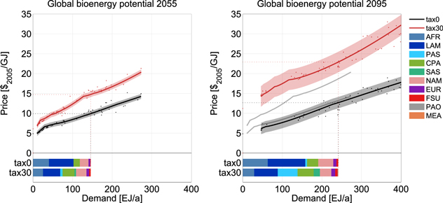
Figure 1. Globally aggregated bioenergy supply curves for 2055 (top left) and 2095 (top right) without (black line) and with a global uniform GHG tax (red line). The gray lines in the 2095 figure (right) indicate the positions of the 2055 supply curves. The colored bars at the bottom show the underlying regional bioenergy production pattern for the sample scenario (145 EJ in 2055 and 240 EJ in 2095). The shaded areas in the upper part indicate the standard deviation of the aggregated fit. Since the fit in 2095 is based on higher demand values than the 2055 fit, the absolute value of the spread is larger in 2095, as is the standard deviation.
Download figure:
Standard image High-resolution imageConditions of bioenergy production differ across regions, as do resulting bioenergy supply curves. Figure 2 shows the regional breakdown of the global supply curve for major producers. Without a GHG tax these are the tropical regions AFR and LAM (figure 1, bottom), which offer access to large areas of forest that can be converted to high-productivity land for crop and bioenergy production. This results in relatively flat supply curves in the tax0 scenario (figure 2, left). CPA and NAM contribute most of the remainder. There are only minor contributions from EUR, FSU, and PAS and almost none from PAO and MEA.
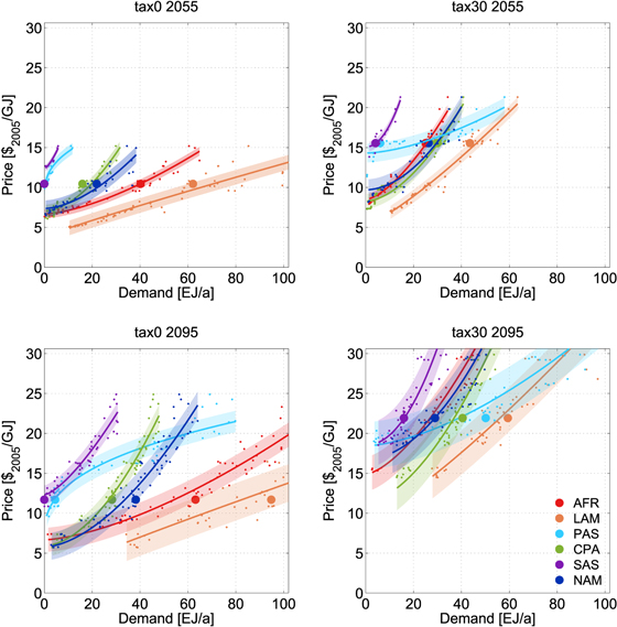
Figure 2. Impact of the GHG tax on the regional supply curves: regional breakdown of the global supply curve for major producers for the tax0 (left) and tax30 scenarios (right), and for 2055 (top) and 2095 (bottom) with the sample scenario marked. The shaded areas indicate the standard deviation of the fit. Since the fit in 2095 includes higher demands than the 2055 fit, the standard deviation is greater.
Download figure:
Standard image High-resolution imageIntroducing a GHG tax changes the relative position of the regional supply curves, since the consequences of pricing emissions are different across regions (figure 2, right). The price-elevating effect can be separated into two components: a steepening of the supply curve due to land exclusion and a translation effect due to non-CO2 co-emissions from bioenergy (supplementary material figure S5). The steepening of the supply curve is caused by the component of the GHG tax that affects the carbon emissions from land conversion (CO2 price), since it effectively stops deforestation (in 2055 and 2095) and thus reduces the amount of land available for the expansion of bioenergy production. The translation effect is caused by pricing nitrogen emissions that accrue from fertilizer use for bioenergy crop cultivation. It does not scale with the bioenergy demand, since the amount of organic and inorganic fertilizer used per unit of bioenergy is constant.
The translation effect applies to the supply curves of all regions (supplementary material figure S6) and is stronger in 2095 than in 2055 since the GHG tax is substantially higher ($1165 versus $165 tCOeq−1). Regions where no forest land is used in the tax0 scenario, such as CPA, PAS, and SAS, are only affected by this N2O-price effect. The supply curves of regions that deforest in the tax0 scenario additionally show a steepening due to CO2 pricing of forest land (strongest in AFR and LAM). The combined effects significantly increase regional supply prices and change the relative position of the supply curves (figure 2). This is reflected in the reallocation of the bioenergy production depicted at the bottom of figure 1: production shifts from AFR and LAM mainly to PAS, CPA, and SAS under the GHG tax. The tax makes PAS competitive, which features a relatively high but flat supply curve. The land restriction in PAS is not as strong as in other regions, since it can expand into productive land that is not under emission control (see below)4 .
4.2. Land and yields
To illustrate the effects of bioenergy demand and GHG tax on processes that drive the allocation and prices of bioenergy, such as changes in land cover, yields, and emissions, the remainder of the analysis focuses on the 2095 results of a medium bioenergy demand scenario selected as a sample out of the full portfolio (2055 results are included in the supplementary material). This is done to keep the analysis comprehensible. The characteristics of the effects observed in other demand scenarios are similar and qualitatively the same. To identify the effect of bioenergy production we compare results of this sample scenario to a zero-demand scenario (see supplementary material figure S4 for the respective scenarios and the full portfolio). Figure 3 shows the global land cover in 2095 and the initial value in 2005 for the four land types that are subject to optimization (top) and their changes from 2005 to 2095 (bottom). Figure 4 depicts the regional breakdown of the changes. Bioenergy production requires substantial amounts of land, almost 500 Mha for 240 EJ in 2095. With and without tax this is predominantly realized by crop land reduction (intensification) and usage of other land.
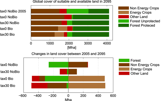
Figure 3. Global cover of land suitable and available (except protected forest) for agricultural production in 2095 with the initial value of 2005 (top). Global changes in land cover between 2005 and 2095 (bottom).
Download figure:
Standard image High-resolution image
Figure 4. Breakdown of the global changes of land cover between 2005 and 2095 into regional changes.
Download figure:
Standard image High-resolution imageWithout a GHG tax bioenergy causes only little additional deforestation (-55 Mha, in LAM mainly), since large amounts of accessible forest are already cleared for food and feed production (−250 Mha), (tax0 Bio versus tax0 NoBio). Bioenergy reduces cropland globally by 300 Mha (−17%) in 2095, mainly in AFR, LAM, CPA, and NAM. The increased usage of other land (−130 Mha) due to bioenergy production in the tax0 Bio scenario has two sources: increased conversion of existing other land (AFR) and usage of land that is abandoned in the tax0 NoBio scenario (LAM, EUR, FSU) (see also figure 4). Under the GHG tax, bioenergy and food production cannot access high-productivity forest land in AFR and LAM since it is effectively protected by the tax. Therefore, bioenergy plantations are partly pushed out of regions that formerly had access to forest (300 Mha in AFR and LAM). In parts this is compensated by further expansion into other land (−100 Mha), since resulting emissions are not penalized by the GHG tax. Substantial amounts of other land are converted in PAS that would have not been touched by the single effect of bioenergy or tax. The remaining part is compensated by the replacement of cropland with bioenergy cropland (−200 Mha), predominantly in SAS. Again, only the combination of bioenergy and tax leads to bioenergy production in SAS.
Bioenergy yields required for the global production of 240 EJ in 2095 vary substantially across regions and range from 80 GJ ha−1 yr−1 (FSU) to 690 GJ ha−1 yr−1 (LAM) in the tax0 scenario and 715 GJ ha−1 yr−1 (PAS) in the tax30 scenario (supplementary material figure S12). While the global average yield remains unchanged at 500 GJ ha−1 yr−1 (27 t ha−1 yr−1), the GHG tax requires substantial yield increases for energy crops in all major producer regions, mostly in PAS (from 300 to 715 GJ ha−1 yr−1), which compensates for the exclusion of productive land in AFR and LAM. If only major producers that cover more than 93% (224 EJ) of the global production (AFR, CPA, LAM, and NAM in the tax0 scenario and additionally PAS and SAS in the tax30 scenario) are taken into account, average yield increases from 596 to 611 GJ ha−1 yr−1 driven by the GHG tax5 . The average yield of regions producing the remaining 17 EJ decreases from 157 to 136 GJ ha−1 yr−1. Further information on yields can be found in the supplementary material.
4.3. Emissions
Figure 5 shows the carbon emissions from the land-use sector cumulated from 2005 to 2095 separated into emissions from food and energy crop production. Without the GHG tax, food production accounts for roughly 234 GtCO2 (80%) of total emissions, mainly caused by deforestation in AFR (120 GtCO2) and LAM (70 GtCO2). Since the GHG tax almost stops deforestation, it substantially reduces carbon emissions from food crop production by 56% (to 102 GtCO2). Remaining carbon emissions are caused by conversion of other land. The production of bioenergy causes additional emissions. If forest is not protected by the GHG tax, bioenergy emissions account for 63 GtCO2, mainly due to deforestation in LAM (40 GtCO2). Under the GHG tax there is no deforestation for bioenergy, but substantial expansion into other land6 , predominantly in PAS (73 GtCO2). This leakage effect increases bioenergy emissions by 54% to 97 GtCO2 cumulated from 2005 to 2095.

Figure 5. CO2 emissions from land-use change due to bioenergy production and other agricultural activities cumulated from 2005 to 2095.
Download figure:
Standard image High-resolution image
5. Discussion and conclusion
We constructed bioenergy supply curves for ten world regions and a global aggregate under full land-use competition using a high-resolution land-use model with endogenous technological change. We find that the implementation of GHG taxes for land-use and land-use change emissions is crucial for the slope of the supply function and the GHG emissions from the land-use sector.
Climate policy not only increases the demand for bioenergy, as several studies show (Rose et al 2013, Calvin et al 2009, Van Vuuren et al 2010a); it could also substantially increase supply prices of biomass raw material, as the present study shows (+$5 GJ−1 in 2055, +$10 GJ−1 in 2095). This is mainly due to the fact that large amounts of high-productivity forest land are de facto excluded by the GHG tax, since expanding into forests would entail substantial carbon emissions and related emission costs. Imposing the GHG tax thus prevents deforestation, lowers carbon emissions, reduces land available for bioenergy production, and increases the opportunity costs of land that is in competition with food production. N2O emissions from fertilizer use further increase bioenergy prices. The GHG tax also reduces the emissions in the case of no bioenergy demand, because the agricultural demand alone is a strong driver for cropland expansion. The bioenergy prices presented in this study emerge under full land-use competition with other crops and are therefore higher than pure production costs on abandoned land found by Hoogwijk et al (2009) and Van Vuuren et al 2009. The potential supply price of biomass raw material is a crucial parameter for the deployment of bioenergy. However, how much and along which conversion routes (e.g. fuels, electricity, heat) bioenergy might be deployed emerges from the balancing of supply and demand, the latter of which is crucially determined by emission reduction targets, carbon prices, biofuel mandates, and technology availability (Mullins et al 2014, Klein et al 2013, Rose et al 2013). Although bioenergy prices presented here may seem high compared to other energy carriers (4.6 $2005 GJ−1 for coal in 2011, IEA 2012b), bioenergy supply at these prices could become relevant, since under climate policy the energy system shows high willingness to pay for bioenergy (Klein et al 2013). The incentive to pay high prices for bioenergy and to create negative emissions from it increases with the carbon price.
Results show that large-scale bioenergy production and high GHG prices, which are likely to coincide under a climate policy that embraces the energy and the land-use sector, can put substantial pressure on the land-use system. In the scenarios of this study bioenergy production requires large amounts of land, predominantly realized by intensification and increased usage of other land. Thus, two measures aiming at climate change mitigation (carbon taxes and bioenergy) could pose a threat to food security since they could dramatically reduce the land available for food production. Although not in the focus of this study, it is important to note that the resulting needs for intensification are likely to increase food prices. However, there is some indication that food-price effects of large-scale bioenergy production could be lower than price effects caused by climate change (Lotze-Campen et al 2013). Adding to a study by Wise et al (2009), who found substantial emissions from deforestation if terrestrial emissions are not priced at all (corresponding to the tax0 scenario used here), this study illustrates the potential consequences of a sectoral fragmented climate policy in the land-use sector: while effectively preventing deforestation the tax cannot prevent considerable carbon emissions resulting from conversion of land that is not covered by the tax or a forest conservation scheme. In our scenarios this is predominantly the case for other land in PAS. Its special role emerges from its high productivity and its high carbon content. Based on data from Erb et al 2007 and FAO 2013 it was accounted 'other land' (cf supplementary material 3.1). Its high carbon content, however, would also justify including it in the forest pool, which would protect it from conversion and thus reduce land-use emissions and alter the supply of bioenergy.
Increased N2O emissions are another adverse effect of bioenergy production reducing the GHG mitigation potential of bioenergy. They are of the same order of magnitude as the CO2 emissions due to bioenergy production. The tax clearly reduces total and bioenergy N2O emissions. The bioenergy emissions comprise emissions from bioenergy production itself (direct) and increased emissions from agriculture resulting from intensification due to bioenergy production (indirect). With the finding that N2O emissions might become a major part of the GHG balance of lignocellulosic biofuels, this study is in line with findings by Melillo et al (2009) and Popp et al (2011b). However, the latter study argues that the substantial negative emissions that could potentially be generated from biomass can overcompensate bioenergy N2O emissions.
The energy yields of bioenergy presented in this study (200 GJ ha−1 yr−1 in 2005, around 600 EJ ha−1 yr−1 in 2055, and up to 700 GJ ha−1 yr−1 in 2095) are at the upper end of the range (130–600 GJ ha−1 yr−1) reported by Haberl et al (2010) for 2055. This partly results from the fact that the model in our study predominantly chooses to produce biomass from herbaceous bioenergy crops (such as Miscanthus), which tend to feature higher yields than woody bioenergy crops (Fischer et al 2005) used in studies presented by Haberl et al (2010). Second, and in contrast to existing studies, bioenergy crop production in the present study competes for cropland with food crop production and thus bio-energy can be grown on highly productive land. Furthermore, the observed prices and underlying production patterns of bioenergy and food crops are based on decisive preconditions in the land-use model, i.e. (i) optimal global allocation of bioenergy and food production and (ii) optimal and timely investments into research and development (R&D) and full impact of R&D on all crops within a region. These optimal conditions are difficult to achieve in the real-world production system, exhibiting underinvestment into research and development (Alston et al 2009), consisting of numerous individual farmers who do not have equal access to technology, and facing land degradation, pests, and changes in weather and climate.
However, the high bioenergy yields at the end of the century are predominantly the result of yield increasing technological progress over almost 90 years. A large part of the yield increases in MAgPIE fills the yield gap between actual yields (observed land-use intensity in the starting year 1995) and the potential yields (derived from the vegetation model LPJmL) that can be achieved under best currently available management conditions. This yield gap can be substantial. For instance, in the regions with the highest yield increases, AFR, LAM, and PAS, the potential yields are reduced to obtain actual yields in 1995 by about 70, 50, and 60% respectively (supplementary material figure S12). MAgPIE bioenergy yields can exceed LPJmL bioenergy yields over time as endogenous investments in R&D push the technology frontier. For AFR, LAM, and PAS the yields in 2095 exceed the potential yields of 1995 by 80, 40, and 20% respectively. Since this study considers endogenous technological change, there is a response in yield growth to the pressure of bioenergy demand and forest conservation. This allows identification of the need for yield growth that would be required if a potential climate change mitigation policy demanded large-scale production of biomass accompanied by GHG prices. Therefore, the development of yields should be interpreted as projections of required yields rather than predictions of expected yields. To what extent they are realistic is currently under discussion. The performance of R&D for second-generation bioenergy crops is highly uncertain. Due to a lack of experience, there are no data available which could be used as a point of reference. Our assumption that yield increases for bioenergy crops will follow yield increases of food crops could be either optimistic or pessimistic. It could be optimistic, since for food crops mainly the corn:shoot ratio was improved and not the overall biomass production (as is required for second-generation bioenergy crops), or it could be pessimistic, since research on lignocellulosic bioenergy crops starts from zero, making it conceivable to assume that there should be a lot of 'low hanging fruits'. Several studies doubt that such high yields could be achieved and argue that the natural productivity poses an upper bound to the production of bioenergy (Haberl et al 2013, Smith et al 2012, Field et al 2008, Erb et al 2012, Campbell et al 2008). Others argue that transferring bioenergy yield levels that were observed under test conditions to huge areas might overestimate the bioenergy potential (Johnston et al 2009). There are also concerns that raising energy crop yields beyond the natural productivity over large regions and over a long time, if possible at all, comes at the costs of increased GHG emissions and other adverse environmental impacts. The findings about bioenergy GHG emissions in the present study (see above) confirm the former at least. There is also doubt that even without bioenergy demand current yield trends will be sufficient to meet the food demand projected for 2050 (Ray et al 2013). On the other hand, Mueller et al (2012) indicate that substantial production increases (up to 70%) are possible by closing the yield gap with currently available management practices.
The following policy relevant conclusions can be drawn from the results. First, a potential climate policy that prices land-use and land-use change emissions could significantly increase supply prices of bioenergy, since it reduces the land available for bioenergy production and since it adds cost for fertilizer emissions to the production costs. Second, a carbon tax can be an effective measure to protect forests (or any other carbon stock under taxation), even if accompanied by large-scale bioenergy production. However, it can only protect land that is defined to be under emission control. The political question of which land to put under carbon taxation defines how much land is accessible. Thus, it is highly relevant not only for the effectiveness of nature conservation and emission mitigation but also for the supply of bioenergy. Third, the combination of the carbon tax and the bioenergy demand is expected to cause substantial pressure and strong intensification on the remaining land, particularly if biomass is produced at large scale. Energy crop yields would be required to rise beyond today's potential yields. A climate policy that builds on carbon taxation and bioenergy deployment thus requires considerable accompanying R&D efforts that ensure continuous technological progress in the agricultural sector.
In this study, we investigated the impact of GHG prices on bioenergy supply. However, there are further crucial factors interacting with the long-term bioenergy supply that could be studied, such as food demand, different levels of forest and biodiversity protection, other land-use based mitigation options (e.g. afforestation), and bioenergy yields. The latter are particularly uncertain, since there is almost no practical experience with large-scale dedicated production of lignocellulosic biomass. Second, due to the potential competition with food production, the impact of bioenergy demand and GHG prices on food supply needs further research. Finally, the issue of fragmented climate policies leading to regionally non-uniform GHG prices and potential emission leakage needs to be considered for the environmental performance of bio-energy production.
Footnotes
- 1
In particular, there is lack of experience with the production of lignocellulosic feedstock for energy purposes, since it has not been produced on a commercial scale yet.
- 2
This range excludes results from Smeets (2007), who reports a potential of 215–1272 EJ yr−1 in 2050 assuming large land area with high productivity.
- 3
Dollars are given as US $2005 in this study. Dollars from other years are converted using the consumer price index http://oregonstate.edu/cla/polisci/sites/default/files/faculty-research/sahr/inflation-conversion/excel/cv2008.xls
- 4
Under the GHG tax the global supply curves begin to flatten from the point where PAS becomes competitive.
- 5
The difference from the global average is mainly due to FSU's low production on large areas of land.
- 6
In cases where bioenergy production inhibits or reverses regrowth of natural vegetation (other land), inhibited negative emissions are counted as positive emissions due to bioenergy production.